The Activation Layer
Introduction
In the previous article, we worked on a new approach, centered on the neural structure, that helps us computing the different elements of the $ Linear $ $ layer $ backward pass.
In this article we will talk about the $ Activation $ $ layer $: one of the last 2 $ layers $ we used in the “Example” introduced in the second article.
The Activation Neural Structure
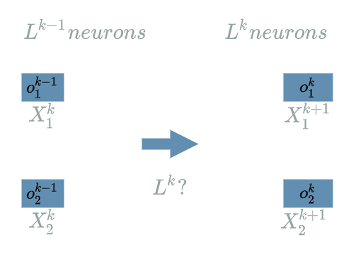
Let us talk about the following setup:
- $ L^{k-1} $ is a $ Linear $ $ layer $ of 2 neurons
- $ L^{k} $ is an $ Activation $ $ layer $
By definition, the $ Activation $ $ layer $ preserves the structure of the previous $ layer $. $ L^{k-1} $ has 2 output neurons, $ L^{k} $ will have 2 output neurons too.
As the $ Activation $ $ layer $ is not a learning layer, it does not declare any weights. We could wonder what the $ Activation $ $ layer $ actually does…
Generally speaking, the $ Activation $ $ layer $ consists in evaluating an $ activation $ function on every input neurons. The choice of the $ activation $ function is up to the developer. Several reasons may justify the use of an $ activation $ function.
-
It allows to transform value ranges. Example: the $ logistic $ $ activation $ function transforms input values in the range of $ [-\infty; \infty] $ to output values in the range of $ [0; 1] $.
\[Logistic(x) = \frac{1}{1 + e^{-x}}\] -
Add a non linearity in the $ model $. $ Heaviside $ example:
\[Heaviside(x) = \left\{\begin{align} 1, & \text{ if $x \geq 0$}\\ 0, & \text{ otherwise} \end{align} \right.\]Note that adding a non linearity after $ layers $ such as the $ Linear $ $ layer $ increases their expressiveness. Let us recap that the final goal is to build a $ model $ that can “understand” data. If $ model $ contains only $ Linear $ $ layers $, the global “understanding” of $ model $ will also be linear. Adding a non linearity increases the spectre of functions that $ model $ is equivalent to.
-
Inspired from the activation potential in biology. $ ReLU $ example:
\[ReLU(x) = \left\{\begin{align} x, & \text{ if $x \geq 0$}\\ 0, & \text{ otherwise} \end{align} \right.\]We will talk about it in the linear function article

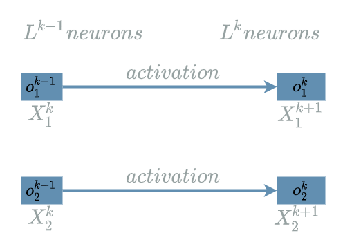
Forward Pass
Just use the $ activation $ function on each input neurons in order to produce the output neurons:
Backward Pass
The $ Activation $ $ layer $ has no weights at all. This means the backward pass will only have to back propagate the learning flow.
Backward Pass for the Learning Flow
We assume we have the same setup as in the first paragraph:
- $ L^{k-1} $ is a $ Linear $ $ layer $ of 2 neurons
- $ L^{k} $ is an $ Activation $ $ layer $
Let us also assume our $ activation $ function is the $ ReLU $ one.
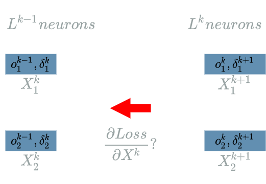
We are currently focusing on the $ L^{k} $ $ layer $, trying to compute:
\[\delta^{k} = \frac{\partial Loss}{\partial X^{k}}(o^{k-1})\]We use the same approach as in the previous article.
The principal idea is to go back to the very structure of $ L^{k} $ in order to find the impacts of $ X^{k} $ on the $ Loss $ function, knowing that the “future” learning flow has already been computed (by definition of the backward pass).
The structure for the $ L^{k} $ $ layer $ is:
- 2 output neurons
- 2 input neurons.
$ \delta^{k+1}_1 $ and $ \delta^{k+1}_2 $ are the “future” learning flow, we must back propagate the learning flow to $ \delta^{k}_1 $ and $ \delta^{k}_2 $.
Computing $ \delta^{k}_1 $
\[\delta^{k}_1 = \frac{\partial Loss}{\partial X^{k}_1}(o^{k-1}_1)\]The interesting variable is $ X^{k}_1 $. There is just one output of $ L^{k} $ that uses $ X^{k}_1 $: $ L^{k}_1 $.
We are now able to build the paths of impacts from $ X^{k}_1 $ to the $ Loss $ function.
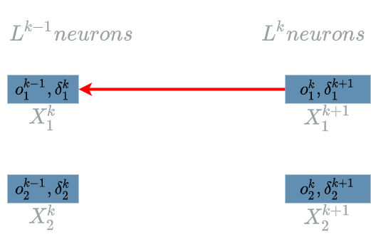
- $ X^{k}_1 $ impacts $ L^{k}_1 $ which impacts the $ Loss $ function
We have only 1 impact, using the chain rule, we obtain the “impact formula”:
\[\delta^{k}_1 = \delta^{k+1}_1 . \frac{\partial L^{k}_1}{X^{k}_1}(o^{k-1}_1)\]We just have to compute:
\[\begin{align} \frac{\partial L^{k}_1}{\partial X^{k}_1} &= \frac{\partial (ReLU(X^{k}_1))}{\partial X^{k}_1} \\ &= \frac{\partial (X^{k}_1 \text{ if } X^{k}_1 \geq 0 \text{ else } 0)}{\partial X^{k}_1} \\ &= 1 \text{ if } X^{k}_1 \geq 0 \text{ else 0 } \end{align}\]Then we evaluate this function on the values that have produced the final $ loss $:
\[\frac{\partial L^{k}_1}{X^{k}_1}(o^{k-1}_1) = 1 \text{ if } o^{k-1}_1 \geq 0 \text{ else 0 }\]We finally use this result in the “impact formula”:
\[\boxed{\delta^{k}_1 = \delta^{k+1}_1 \text{ if } o^{k-1}_1 \geq 0 \text{ else 0 }}\]Computing $ \delta^{k}_2 $
Same as in the previous paragraph. The result is:
\[\boxed{\delta^{k}_2 = \delta^{k+1}_2 \text{ if } o^{k-1}_2 \geq 0 \text{ else 0 }}\]Example
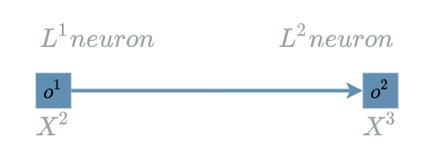
We have already used an $ Activation $ $ layer $ in the “Example” of the previous articles. Let us have a look at the $ model $ we used in the weights article:
\[\begin{align} L1(X^1) &= X^1 & \text{ with } X^1 = (X^1_1, X^1_2, X^1_3) \\ L2(X^2, W^2) &= W^2 . X^2 & \text{ with } X^2 = (X^2_1, X^2_2, X^2_3) \\ & & \text{ and } W^2 = (W^2_1, W^2_2, W^2_3) \\ &= W^2_1 . X^2_1 + W^2_2 . X^2_2 + W^2_3 . X^2_3 \\ L3(X^3) &= X^3 \text{ if } X^3 \geq 0 \text{ else } 0 \\ \\ model(X) &= L3(L2(L1(X))) & \text{ with } X = (X_1, X_2, X_3) \\ Loss(X^4, Y^{truth}) &= \frac{1}{2} (X^4 - Y^{truth})^2 \end{align}\]$ L3 $ is indeed an $ Activation $ $ layer $. Its neural structure is simple: it has just 1 output neuron.
Forward Pass for L3
By definition, we just have to use the $ L3 $ explicit formula:
\[L3(X^3) = X^3 \text{ if } X^3 \geq 0 \text{ else } 0\]Backward Pass for L3
In the backward pass for the learning flow, we found:
\[\boxed{\delta^{k}_1 = \delta^{k+1}_1 \text{ if } o^{k-1}_1 \geq 0 \text{ else 0 }}\] \[\boxed{\delta^{k}_2 = \delta^{k+1}_2 \text{ if } o^{k-1}_2 \geq 0 \text{ else 0 }}\]We adjust these formula to the current neural structure:
\[\delta^{3} = \delta^{4} \text{ if } o^2 \geq 0 \text{ else 0 }\]which is what we already computed in the backward pass article.
Conclusion
We have seen the neural structure for the $ Activation $ $ layer $.
Let us talk about the $ Input \text{ } 1D $ $ layer $ in the next article.