The Convolution Layer
Introduction
In the previous article, we explored how to build representations when the data input are images: we introduced the $ Convolution $ $ layer $. We used convolution kernels that capture spatial information of the channel they are associated to.
The question is now: how can the $ Convolution $ $ layer $ learn anything ?
The Convolution Neural Structure
We will work the same way as in the linear article, introducing the $ Convolution $ neural structure.
Before that, let us recall the diagram of the $ Convolution $ operation we saw at the previous article.
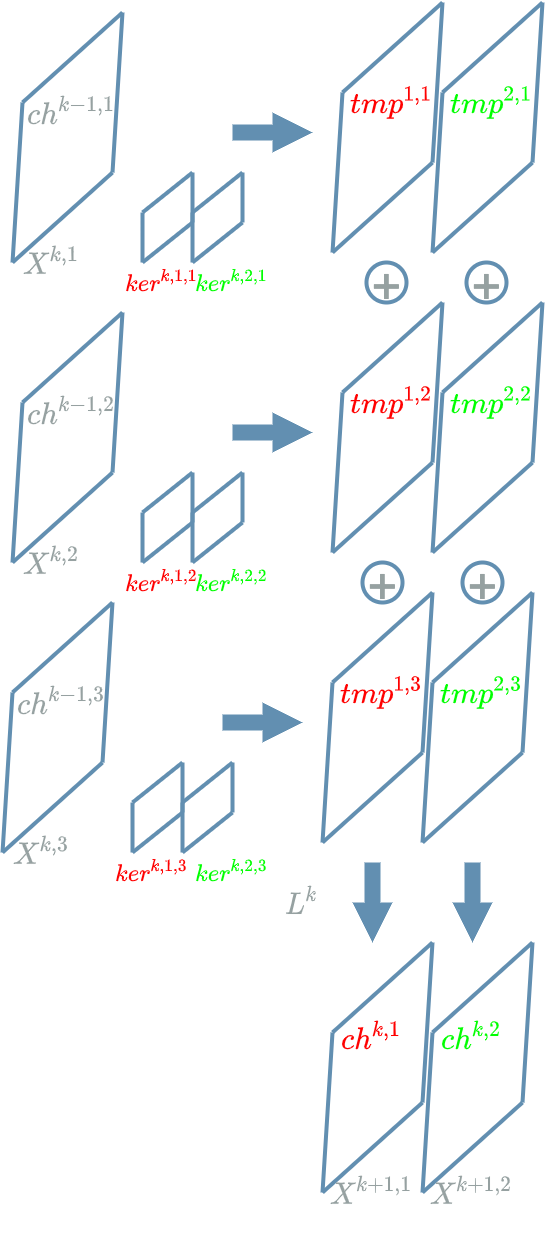
In order to fix the ideas the diagram above shows an example $ L^k $ $ Convolution $ $ layer $ where $ ch^{k-1,1} $, $ ch^{k-1,2} $, $ ch^{k-1,3} $ are the 3 input channels and $ ch^{k,1} $ and $ ch^{k,2} $ are the two output channels. Note that we use 6 different convolution kernels that correspond to the combination: $ 2 \textbf{ output channels } * 3 \textbf{ input channels } = 6 $.
In the following we will zoom in this part of the previous diagram:
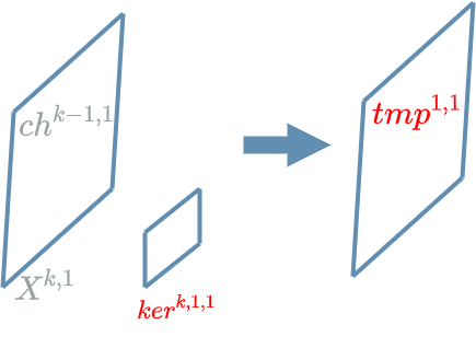
The elements we called “pixels” in the previous article are in fact the neurons of our $ Convolution $ $ layer $. Applying the convolution kernel $ k^{1,1} $ to the grid of neurons of our input channel $ ch^{k-1,1} $ allows us to compute a grid of temporary neurons $ tmp^{1,1} $.
Now let us zoom on the computation of one temporary neuron \(tmp^{1,1}_{4,4}\). In order to simplify the diagram, we get rid of some indices, keeping only the indices relating to the positions in the grid. We want to compute $ tmp_{4,4} $.
From what we saw in the previous article, we know how to proceed: we take the center of our $ ker $ kernel ($ ker_{1,1} $ as $ ker $ is a kernel of size (3,3) in our example), we align it with the neuron in the input channel ($ ch_{3, 3} $ as $ ch $ is a grid of size (7,7) in our example) and we add the different multiplied couples together.
Here are the different multiplied couples:
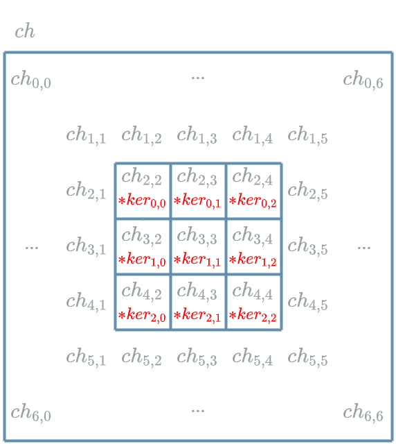
And here we add them together to obtain:
\[\begin{align} tmp_{4,4} &= & (ch_{2,2} * ker_{0,0}) + (ch_{2,3} * ker_{0,1}) + (ch_{2,4} * ker_{0,2}) \\ & & + (ch_{3,2} * ker_{1,0}) + (ch_{3,3} * ker_{1,1}) + (ch_{3,4} * ker_{1,2}) \\ & & + (ch_{4,2} * ker_{2,0}) + (ch_{4,3} * ker_{2,1}) + (ch_{4,4} * ker_{2,2}) \end{align}\]Now let us zoom out. We have just computed one temporary neuron $ tmp^{1,1}_{4,4} $. We have to do the same to compute every temporary neuron of $ tmp^{1,1} $.
Let us zoom out again: we have computed one temporary grid $ tmp^{1,1} $, we have to do the same to compute the other temporary grids with the other combinations: $ ch^{k-1,1} $ and $ ker^{k,2,1} $ to obtain $ tmp^{2,1} $, $ ch^{k-1,2} $ and $ ker^{k,2,2} $ to obtain $ tmp^{2,2} $, $ ch^{k-1,3} $ and $ ker^{k,1,3} $ to obtain $ tmp^{1,3} $, $ ch^{k-1,3} $ and $ ker^{k,2,3} $ to obtain $ tmp^{2,3} $.
Finally it is simple to obtain the output channels, each being a grid of output neurons:
\[\boxed{ \begin{align} ch^{k,1} = tmp^{1,1} + tmp^{1,2} + tmp^{1,3} + b^{k,1}\\ ch^{k,2} = tmp^{2,1} + tmp^{2,2} + tmp^{2,3} + b^{k,2} \end{align} }\]where $ b^{k,1} $ and $ b^{k,1} $ are biases.
Looking at one particular neuron of the grid, for example $ ch^{k,1}_{4,4} $ we have:
\[\begin{align} ch^{k,1}_{4,4} &= & (ch^{k-1,1}_{2,2} * ker^{k,1,1}_{0,0}) + (ch^{k-1,1}_{2,3} * ker^{k,1,1}_{0,1}) + (ch^{k-1,1}_{2,4} * ker^{k,1,1}_{0,2}) \\ & & + (ch^{k-1,1}_{3,2} * ker^{k,1,1}_{1,0}) + (ch^{k-1,1}_{3,3} * ker^{k,1,1}_{1,1}) + (ch^{k-1,1}_{3,4} * ker^{k,1,1}_{1,2}) \\ & & + (ch^{k-1,1}_{4,2} * ker^{k,1,1}_{2,0}) + (ch^{k-1,1}_{4,3} * ker^{k,1,1}_{2,1}) + (ch^{k-1,1}_{4,4} * ker^{k,1,1}_{2,2}) \\ \\ & & + (ch^{k-1,2}_{2,2} * ker^{k,1,2}_{0,0}) + (ch^{k-1,2}_{2,3} * ker^{k,1,2}_{0,1}) + (ch^{k-1,2}_{2,4} * ker^{k,1,2}_{0,2}) \\ & & + (ch^{k-1,2}_{3,2} * ker^{k,1,2}_{1,0}) + (ch^{k-1,2}_{3,3} * ker^{k,1,2}_{1,1}) + (ch^{k-1,2}_{3,4} * ker^{k,1,2}_{1,2}) \\ & & + (ch^{k-1,2}_{4,2} * ker^{k,1,2}_{2,0}) + (ch^{k-1,2}_{4,3} * ker^{k,1,2}_{2,1}) + (ch^{k-1,2}_{4,4} * ker^{k,1,2}_{2,2}) \\ \\ & & + (ch^{k-1,3}_{2,2} * ker^{k,1,3}_{0,0}) + (ch^{k-1,3}_{2,3} * ker^{k,1,3}_{0,1}) + (ch^{k-1,3}_{2,4} * ker^{k,1,3}_{0,2}) \\ & & + (ch^{k-1,3}_{3,2} * ker^{k,1,3}_{1,0}) + (ch^{k-1,3}_{3,3} * ker^{k,1,3}_{1,1}) + (ch^{k-1,3}_{3,4} * ker^{k,1,3}_{1,2}) \\ & & + (ch^{k-1,3}_{4,2} * ker^{k,1,3}_{2,0}) + (ch^{k-1,3}_{4,3} * ker^{k,1,3}_{2,1}) + (ch^{k-1,3}_{4,4} * ker^{k,1,3}_{2,2}) \\ \\ & & + b^{k,1} \end{align}\]The Machine Learning Paradigm
The different neurons in the grid correspond to the output of the $ Convolution $ $ layer $. Looking back at the linear layer article, the neurons were structured as vector of numbers. It seems legitimate that our output are now grids.
Still, we are looking for a “moving part”, such as the weights we introduced in the weights article. We have a perfect place to consider weights variables in our $ Convolution $ $ layer $, right in the convolution kernels.
This enables us not to choose these kernels at all and rely on the learning process operating during the gradient descent algorithm (see this article). In a way, it is the data that will configure those kernels “automatically”.
This is the beautiful paradigm of the machine learning. We try to give the $ models $ the power to configure the required operations in order to correctly “understand” the data.
Yet, for now, we must also
keep in mind that we do not give that much power to these $ models $. We actually are just talking about some
“moving part” parameters, the weights, that allow to configure some specific $ layers $. For now these
specific $ layers $ are: the linear layer and the $ Convolution $ $ layer $.
We see that in fact, the global structure of the $ models $
(the structure in $ layers $, the number of $ layers $, the nature of each $ layer $…)
is still up to the developer ![]()
Forward Pass
We have already seen how the $ Convolution $ $ layer $ computes its forward pass, it merely consists in applying the operation described in the previous paragraph.
Backward Pass for the Learning Flow
Let us focus on the computation of the learning flow for the central input neuron of our $ L^{k} $ $ Convolution $ $ layer $:
\[\delta^{k,1}_{3,3} = \frac{\partial Loss}{\partial X^{k,1}_{3,3}}(ch^{k-1,1}_{3,3})\]The interesting variable is $ X^{k,1}_{3,3} $, nearly visible in the input grid in this diagram. Let us find its impacts on the $ Loss $ function.
What is difficult in the $ Convolution $ case is the dual operation we saw in the previous article:
- the spatial context which is captured by the convolution kernels (this is specific to the 2D case)
- the combination of previous representations (this is a legacy of the 1D case)
We are trying to resolve the impacts of $ X^{k,1}_{3,3} $ on the output grids of our $ L^{k} $ $ layer $. Let us consider the diagram below coming from the forward pass.
What is important is to note that during the forward pass, there are multiple output neurons that have captured the spatial context from the neuron we are studying $ ch^{k-1,1}_{3,3} $ during their own computation. This is due to the 1st point.
For example, let us apply our $ ker^{k,1,1} $ convolution kernel on \(ch^{k-1,1}_{2,2}\) in order to obtain \(ch^{k,1}_{2,2}\). We see that one of the “multiplied couple” is \(ch^{k-1,1}_{3,3} * ker^{k,1,1}_{2,2}\). This means that \(ch^{k-1,1}_{3,3}\) impacts \(ch^{k,1}_{2,2}\).
But due to the 2nd point, we should also try to apply our \(ker^{k,2,1}\) convolution kernel on \(ch^{k-1,1}_{2,2}\) in order to obtain \(ch^{k,2}_{2,2}\). We see that one of the “multiplied couple” is \(ch^{k-1,1}_{3,3} * ker^{k,2,1}_{2,2}\). This means that \(ch^{k-1,1}_{3,3}\) also impacts \(ch^{k,2}_{2,2}\).
For now, we have found 2 output neurons of $ L^{k} $ that are impacted by \(ch^{k-1,1}_{3,3}\): \(ch^{k,1}_{2,2}\) and \(ch^{k,2}_{2,2}\).
In fact there are other impacts ! Due to the 1st point here is the list of the neurons that capture context from $ ch^{k-1,1}_{3,3} $:
\[\begin{matrix} ch^{k-1,1}_{2,2} & ch^{k-1,1}_{2,3} & ch^{k-1,1}_{2,4} \\ ch^{k-1,1}_{3,2} & ch^{k-1,1}_{3,3} & ch^{k-1,1}_{3,4} \\ ch^{k-1,1}_{4,2} & ch^{k-1,1}_{4,3} & ch^{k-1,1}_{4,4} \end{matrix}\]Due to the 2nd point here is the list of the output neurons that have used these input neurons:
\[\begin{matrix} ch^{k,1}_{2,2} & ch^{k,1}_{2,3} & ch^{k,1}_{2,4} \\ ch^{k,1}_{3,2} & ch^{k,1}_{3,3} & ch^{k,1}_{3,4} \\ ch^{k,1}_{4,2} & ch^{k,1}_{4,3} & ch^{k,1}_{4,4} \end{matrix}\] \[\begin{matrix} ch^{k,2}_{2,2} & ch^{k,2}_{2,3} & ch^{k,2}_{2,4} \\ ch^{k,2}_{3,2} & ch^{k,2}_{3,3} & ch^{k,2}_{3,4} \\ ch^{k,2}_{4,2} & ch^{k,2}_{4,3} & ch^{k,2}_{4,4} \end{matrix}\]We have found $ 2 * 9 = 18 $ output neurons that are impacted by $ ch^{k-1,1}_{3,3} $ !
We add these 18 impacts, using the chain rule and the “future” learning flow to obtain the “impact formula”:
\[\begin{align} \delta^{k,1}_{3,3} &= & \delta^{k+1,1}_{2,2} . \frac{\partial X^{k+1,1}_{2,2}}{\partial X^{k,1}_{3,3}}(ch^{k-1,1}_{2,2}) + \delta^{k+1,1}_{2,3} . \frac{\partial X^{k+1,1}_{2,3}}{\partial X^{k,1}_{3,3}}(ch^{k-1,1}_{2,3}) \\ & & + ... \\ & & + \delta^{k+1,2}_{2,2} . \frac{\partial X^{k+1,2}_{2,2}}{\partial X^{k,1}_{3,3}}(ch^{k-1,2}_{2,2}) + \delta^{k+1,2}_{2,3} . \frac{\partial X^{k+1,2}_{2,3}}{\partial X^{k,1}_{3,3}}(ch^{k-1,2}_{2,3}) \\ & & + ... \end{align}\]Let us compute one of these:
\[\begin{align} \frac{\partial X^{k+1,1}_{2,2}}{X^{k,1}_{3,3}}(ch^{k-1,1}_{2,2}) &= \frac{\partial (... + X^{k,1}_{3,3} * Ker^{k,1,1}_{2,2} + ... + B^{k,1})}{\partial X^{k,1}_{3,3}}(ch^{k-1,1}_{2,2}) \\ &= ker^{k,1,1}_{2,2} \end{align}\]We obtain our final “impact formula”:
\[\boxed{ \begin{align} \delta^{k,1}_{3,3} &= & \delta^{k+1,1}_{2,2} . ker^{k,1,1}_{2,2} + \delta^{k+1,1}_{2,3} . ker^{k,1,1}_{2,1} \\ & & + ... \\ & & + \delta^{k+1,2}_{2,2} . ker^{k,2,1}_{2,2} + \delta^{k+1,2}_{2,3} . ker^{k,2,1}_{2,1} \\ & & + ... \end{align} }\]We have just computed the information flow for one of the input neurons: $ \delta^{k,1}_{3,3} $. We have to do the same for every other input neurons of the first channel and then repeat for the other channels: $ \delta^{k,2} $ and $ \delta^{k,3} $.
Backward Pass for the Weights
As we mentioned in the machine learning paradigm paragraph, the weights of our $ Convolution $ $ layer $ are the different elements of its convolution kernels.
Let us focus on the computation of $ \delta ker^{k,1,1}_{0,0} $:
\[\delta ker^{k,1,1}_{0,0} = \frac{\partial Loss}{\partial Ker^{k,1,1}_{0,0}}(ch^{k-1,1})\]We are trying to resolve the impacts of $ Ker^{k,1,1}_{0,0} $ on the output grids of our $ L^{k} $ $ layer $.
Looking back at the first diagram, there is just one output grid that is using $ ker^{k,1,1} $, it is $ ch^{k,1} $ (going through the intermediate channel $ tmp^{1,1} $).
But for this unique output grid, there are multiple output neurons that have been computed using $ ker^{k,1,1}_{0,0} $.
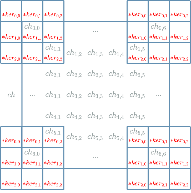
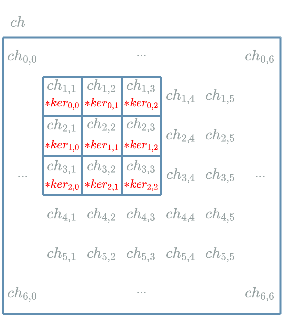
Let us apply our $ ker^{k,1,1} $ convolution kernel on \(ch^{k-1,1}_{0,0}\) in order to obtain \(ch^{k,1}_{0,0}\). We see that the “multiplied couple” associated with \(ker^{k,1,1}_{0,0}\) is 0 which means that \(ker^{k,1,1}_{0,0}\) does not impact $ ch^{k,1}_{0,0} $.
If we apply our $ ker^{k,1,1} $ convolution kernel on \(ch^{k-1,1}_{6,6}\) in order to obtain \(ch^{k,1}_{6,6}\), we see that the “multipled couple” associated with \(ker^{k,1,1}_{0,0}\) is not 0 which means that \(ker^{k,1,1}_{0,0}\) impacts \(ch^{k,1}_{6,6}\).
We see $ ker^{k,1,1}_{0,0} $ impacts many output neurons : the whole output grid $ ch^{k,1} $ except for the top row and the left column. This does $ 7 * 7 - 7 - 6 = 36 $ impacts !
We add these 36 impacts, using the chain rule and the “future” learning flow to obtain the “impact formula”:
\[\begin{align} \delta ker^{k,1,1}_{0,0} &= & \delta^{k+1,1}_{1,1} . \frac{\partial X^{k+1,1}_{1,1}}{\partial Ker^{k,1,1}_{0,0}}(ch^{k-1,1}_{1,1}) + \delta^{k+1,1}_{1,2} . \frac{\partial X^{k+1,1}_{1,2}}{\partial Ker^{k,1,1}_{0,0}}(ch^{k-1,1}_{1,2}) \\ & & + ... + \delta^{k+1,1}_{1,6} . \frac{\partial X^{k+1,1}_{1,6}}{\partial Ker^{k,1,1}_{0,0}}(ch^{k-1,1}_{1,6}) \\ & & + ... \\ & & + \delta^{k+1,1}_{6,1} . \frac{\partial X^{k+1,1}_{6,1}}{\partial Ker^{k,1,1}_{0,0}}(ch^{k-1,1}_{6,1}) + \delta^{k+1,1}_{6,2} . \frac{\partial X^{k+1,1}_{6,2}}{\partial Ker^{k,1,1}_{0,0}}(ch^{k-1,1}_{6,2}) \\ & & + ... + \delta^{k+1,1}_{6,6} . \frac{\partial X^{k+1,1}_{6,6}}{\partial Ker^{k,1,1}_{0,0}}(ch^{k-1,1}_{6,6}) \end{align}\]Let us compute one of these:
\[\begin{align} \frac{\partial X^{k+1,1}_{6,6}}{\partial Ker^{k,1,1}_{0,0}}(ch^{k-1,1}_{6,6}) &= \frac{\partial (... + X^{k,1}_{5,5} * Ker^{k,1,1}_{0,0} + ... + B^{k,1})}{\partial Ker^{k,1,1}_{0,0}}(ch^{k-1,1}_{6,6}) \\ &= ch^{k-1,1}_{5,5} \end{align}\]We obtain our final “impact formula”:
\[\boxed{ \begin{align} \delta ker^{k,1,1}_{0,0} &= & \delta^{k+1,1}_{1,1} . ch^{k-1,1}_{0,0} + \delta^{k+1,1}_{1,2} . ch^{k-1,1}_{0,1} + ... + \delta^{k+1,1}_{1,6} . ch^{k-1,1}_{0,5} \\ & & + ... \\ & & + \delta^{k+1,1}_{6,1} . ch^{k-1,1}_{5,0} + \delta^{k+1,1}_{6,2} . ch^{k-1,1}_{5,1} + ... + \delta^{k+1,1}_{6,6} . ch^{k-1,1}_{5,5} \end{align} }\]We have just computed the opposite direction to follow for $ ker^{k,1,1}_{0,0}$ update. We have to do the same for every other weights of $ ker^{k,1,1} $ and then repeat for the other convolution kernels: $ ker^{k,2,1} $, $ ker^{k,1,2} $, $ ker^{k,2,2} $, $ ker^{k,1,3} $ and $ ker^{k,2,3} $.
Backward Pass for the Biases
Let us focus on the computation of $ \delta b^{k,1} $.
We are trying to resolve the impacts of $ B^{k,1} $ on the output grids of our $ L^{k} $ $ layer $.
Looking back at the first diagram, there is just one output grid that is using $ b^{k,1} $, it is $ ch^{k,1} $.
But for this unique output grid, there are multiple output neurons that have been computed using $ b^{k,1} $. This time every neuron of $ ch^{k,1} $ is impacted by $ b^{k,1} $: this does $ 7 * 7 = 49 $ impacts !
We add these 49 impacts, using the chain rule and the “future” learning flow to obtain the “impact formula”:
\[\begin{align} \delta b^{k,1} &= & \delta^{k+1,1}_{0,0} . \frac{\partial X^{k+1,1}_{0,0}}{\partial B^{k,1}}(ch^{k-1,1}_{0,0}) + \delta^{k+1,1}_{0,1} . \frac{\partial X^{k+1,1}_{0,1}}{\partial B^{k,1}}(ch^{k-1,1}_{0,1}) \\ & & + ... + \delta^{k+1,1}_{0,6} . \frac{\partial X^{k+1,1}_{0,6}}{\partial B^{k,1}}(ch^{k-1,1}_{0,6}) \\ & & + ... \\ & & + \delta^{k+1,1}_{6,0} . \frac{\partial X^{k+1,1}_{6,0}}{\partial B^{k,1}}(ch^{k-1,1}_{6,0}) + \delta^{k+1,1}_{6,1} . \frac{\partial X^{k+1,1}_{6,1}}{\partial B^{k,1}}(ch^{k-1,1}_{6,1}) \\ & & + ... + \delta^{k+1,1}_{6,6} . \frac{\partial X^{k+1,1}_{6,6}}{\partial B^{k,1}}(ch^{k-1,1}_{6,6}) \end{align}\]Let us compute one of these:
\[\begin{align} \frac{\partial X^{k+1,1}_{0,0}}{\partial B^{k,1}}(ch^{k-1,1}_{0,0}) &= \frac{\partial (... + B^{k,1})}{\partial B^{k,1}}(ch^{k-1,1}_{0,0}) \\ &= 1 \end{align}\]We obtain our final “impact formula”:
\[\boxed{ \begin{align} \delta b^{k,1} &= & \delta^{k+1,1}_{0,0} + \delta^{k+1,1}_{0,1} + ... + \delta^{k+1,1}_{0,6} \\ & & + ... \\ & & + \delta^{k+1,1}_{6,0} + \delta^{k+1,1}_{6,1} + ... + \delta^{k+1,1}_{6,6} \end{align} }\]We have just computed the opposite direction to follow for $ b^{k,1} $ update. We do the same for $ b^{k,2} $.
Conclusion
We have seen the neural structure for the $ Convolution $ $ layer $. In the next article we will see a simple $ layer $ that will help us create our first real deep learning $ model $ !