The Input 1D Layer
Introduction
In the previous article, we talked about the $ Activation $ $ layer $.
In this article we will talk about the $ Input \text{ } 1D $ $ layers $: the last $ layer $ we used in the “Example” introduced in the second article.
The Input 1D Neural Structure
As we have seen in the second article, the input layer is the first $ layer $ of the $ model $. It directly receives the data given by the developer.
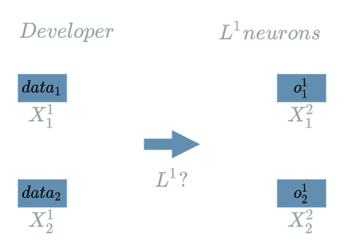
Still, it has a neural structure. For example let us suppose $ L^{1} $ is an $ Input \text{ } 1D $ $ layer $ with 2 output neurons:
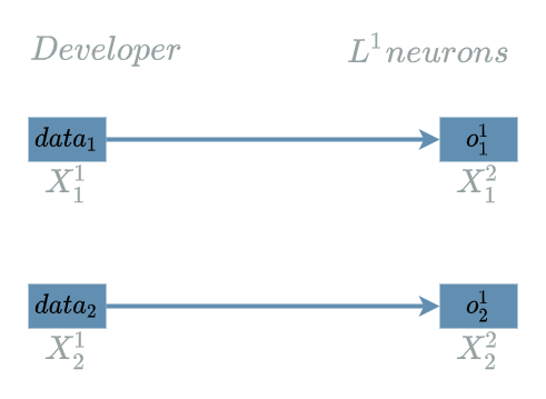
Forward Pass
In fact, it just consists in storing the data given by the developer inside the output neurons:
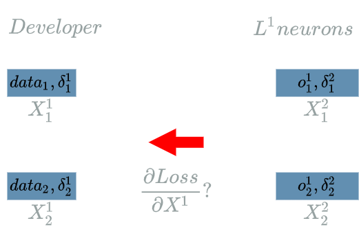
Backward Pass for the Learning Flow
We assume $ L1 $ is an $ Input \text{ } 1D $ $ layer $ that produces 2 output neurons. We are trying to compute:
\[\delta^{1} = \frac{\partial Loss}{\partial X^{1}}(data)\]Let us find the impacts of $ X^{1} $ on the $ Loss $ function, knowing that the “future” learning flow has already been computed (by definition of the backward pass).
The structure for the $ L^{1} $ $ layer $ is:
- 2 output neurons
- 2 input neurons.
$ \delta^{2}_1 $ and $ \delta^{2}_2 $ are the “future” learning flow, we must back propagate the learning flow to $ \delta^{1}_1 $ and $ \delta^{2}_2 $.
Computing $ \delta^{1}_1 $
\[\delta^{1}_1 = \frac{\partial Loss}{\partial X^{1}_1}(data_1)\]The interesting variable is $ X^{1}_1 $. There is just one output of $ L^{1} $ that uses $ X^{1}_1 $: $ L^{1}_1 $.
We are now able to build the paths of impacts from $ X^{1}_1 $ to the $ Loss $ function.
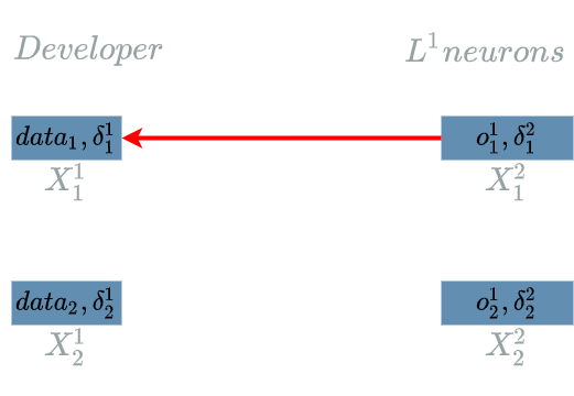
- $ X^{1}_1 $ impacts $ L^{1}_1 $ which impacts the $ Loss $ function
We have only 1 impact, using the chain rule, we obtain the “impact formula”:
\[\delta^{1}_1 = \delta^{2}_1 . \frac{\partial L^{1}_1}{X^{1}_1}(data_1)\]We just have to compute:
\[\begin{align} \frac{\partial L^{1}_1}{\partial X^{1}_1} &= \frac{\partial (L^{1}(X^{1}_1))}{\partial X^{1}_1} \\ &= \frac{\partial (X^{1}_1)}{\partial X^{1}_1} \\ &= 1 \end{align}\]Then we evaluate this function on the values that have produced the final $ loss $:
\[\frac{\partial L^{1}_1}{X^{1}_1}(data_1) = 1\]We finally use this result in the “impact formula”:
\[\boxed{\delta^{1}_1 = \delta^{2}_1}\]Computing $ \delta^{k}_2 $
Same as in the previous paragraph. The result is:
\[\boxed{\delta^{1}_2 = \delta^{2}_2}\]Example
We have already used an $ Input \text{ } 1D $ $ layer $ in the “Example” of the previous articles. Let us have a look at the $ model $ we used in the weights article:
\[\begin{align} L1(X^1) &= X^1 & \text{ with } X^1 = (X^1_1, X^1_2, X^1_3) \\ L2(X^2, W^2) &= W^2 . X^2 & \text{ with } X^2 = (X^2_1, X^2_2, X^2_3) \\ & & \text{ and } W^2 = (W^2_1, W^2_2, W^2_3) \\ &= W^2_1 . X^2_1 + W^2_2 . X^2_2 + W^2_3 . X^2_3 \\ L3(X^3) &= X^3 \text{ if } X^3 \geq 0 \text{ else } 0 \\ \\ model(X) &= L3(L2(L1(X))) & \text{ with } X = (X_1, X_2, X_3) \\ Loss(X^4, Y^{truth}) &= \frac{1}{2} (X^4 - Y^{truth})^2 \end{align}\]$ L1 $ is indeed an $ Input \text{ } 1D $ $ layer $. Its neural structure is simple: it has 3 output neurons.
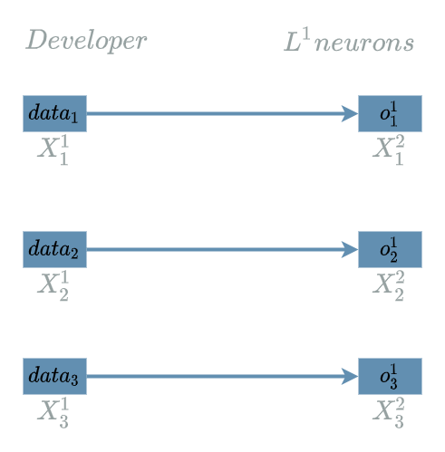
Forward Pass for L1
By definition, we just have to use the $ L1 $ explicit formula:
\[L1(X^1) = X^1\]Backward Pass for L1
In the backward pass for the learning flow, we found:
\[\boxed{\delta^{1}_1 = \delta^{2}_1}\] \[\boxed{\delta^{1}_2 = \delta^{2}_2}\]We can summarize these formula for the current neural structure:
\[\delta^{1} = \delta^{2}\]which is what we already computed in the backward pass article.
Conclusion
We have seen the neural structure for each and every $ layer $ that appeared in the “Example” we introduced in the second article.
We are now ready to go back to the very simple $ model $ and illustrate the weights update process
in the next article ![]()