The Linear Layer

Introduction

In the previous chapter, we explored the general concepts of the deep learning machinery. We saw that the deep learning $ model $ is at the core of everything. Inside the model, we found a graph of ordered $ layers $ which may contain some weights. These weights are the most prominent part and their update is directly responsible for the learning process itself. We saw this learning process in action during the gradient descent algorithm and we finally saw an upgraded version of it thanks to batch learning.

In this chapter, we will explore the different $ layers $ deeper. This will help us knowing how to choose the best $ layers $ in order to design our future deep learning $ models $. The main characteristic of these $ layers $ is whether they have weights or not. As the weights are directly implied in the learning process, the $ layers $ with weights will be involved in the process of building representations (first referenced here) while the $ layers $ with no weights will be passive.

In both cases, the $ layers $ two main operations during the learning process are the forward pass and the backward pass. As we saw in the backward pass article, each $ layer $ propagates the information flow during the forward pass and the learning flow during the backward pass. This backward pass implies some computations that proved to be painful. This chapter will enable us to explain this back propagation with a new perspective: the $ layer $’s neural structure.

Let us begin with the $ Linear $ $ layer $…

The Linear Neural Structure

In order to better understand the function realized by one $ Linear $ $ layer $, we will explore its neural structure.

Let us take a $ L^{k} $ $ Linear $ $ layer $. As every $ Linear $ $ layer $ it is a learning $ layer $, which means it declares weights (see the weights article). Let us note $ W^{k} $ these weights.

By definition of the forward pass (see this article) we need $ L^{k} $’s previous layer $ L^{k-1} $ in order to evaluate $ L^{k} $ on the outputs of $ L^{k-1} $. For now this is how we represent this relation:

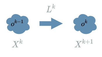
In the diagram, we are now ready to remove the clouds and turn them into neurons! Each neuron represents an $ X $ variable.

But there is more… In the weights article, we saw how the learning flow is necessary to compute the directions of the weights’ update. And in the backward pass article, we saw that the learning flow depends on the “future” learning flow and the “previous” outputs. This is the reason why we actually put some values in the clouds in our different diagrams: these values must be stored during the current couple of forward pass and backward pass. Thus, we will now store these values inside the neurons.

Let us go back to our $ L^k $ $ Linear $ $ layer $ and suppose it has 2 neurons. This literally means $ L^{k} $ produces 2 outputs: $ o^{k}_1 $ and $ o^{k}_2 $.

Let us suppose $ L^{k-1} $ produces 3 output neurons: $ o^{k-1}_1 $, $ o^{k-1}_2 $ and $ o^{k-1}_3 $.

The diagram becomes:

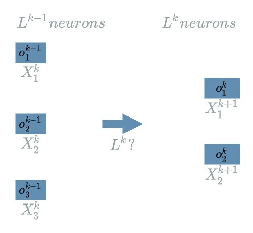
Note that the number of neurons for each $ layer $ is up to the developer. The fact that we chose 2 output neurons for $ L^{k} $ and 3 output neurons for $ L^{k-1} $ is just an example. We could have also decided that $ L^{k} $ produces 20 945 output neurons but it would have been less practical to draw the diagram.

The final question is: what is the form of the $ L^{k} $ function ? We just know it transforms the outputs of $ L^{k-1} $ into the very own outputs of $ L^{k} $.

The answer is: we do not “exactly” know

This is the reason why we do some crazy move: connecting each $ L^{k-1} $ neuron to each $ L^{k} $ neuron. The connexions being assured by the weights of $ L^{k} $: $ W^{k} $. That way, the values of the weights will be adjusted during the training phase (see the weights article), modifying the function $ L^{k} $ itself so that it actually performs the “right” transformation on the $ L^{k-1} $ outputs in order to minimize the $ Loss $ function.

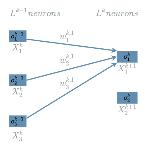
But there is one subtlety here: $ L^{k} $ has two neurons. So each $ L^{k} $ neuron will be connected to every neurons of $ L^{k-1} $. This is the main characteristic of the $ Linear $ $ layer $: connecting every output neurons to every input neurons.

Concretely, we must declare $ W^{k, 1} $ weights that will connect the different input neurons: $ o^{k-1}_1 $, $ o^{k-1}_2 $ and $ o^{k-1}_3 $ to the first output neuron $ o^{k}_1 $.

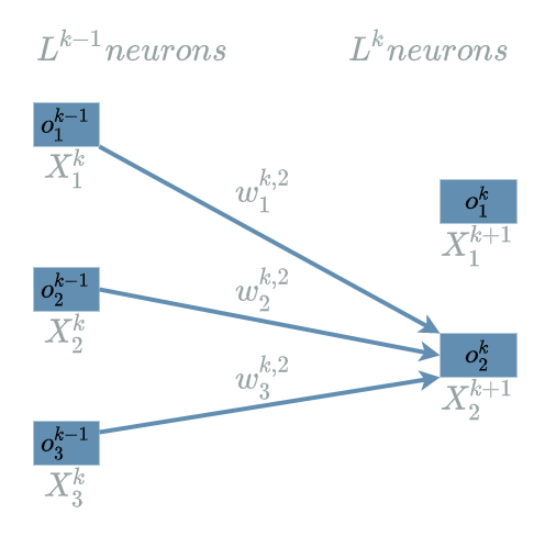
And we must also declare $ W^{k, 2} $ weights that will connect the different input neurons: $ o^{k-1}_1 $, $ o^{k-1}_2 $ and $ o^{k-1}_3 $ to the second output neuron $ o^{k}_2 $.

Forward Pass

Using the same $ L^{k} $ $ layer $ as in the previous paragraph, we have:

\[\begin{align} L^{k}_1(X^{k}) &= W^{k, 1}_1 . X^{k}_1 + W^{k, 1}_2 . X^{k}_2 + W^{k, 1}_3 . X^{k}_3 + B^{k}_1 \\ L^{k}_2(X^{k}) &= W^{k, 2}_1 . X^{k}_1 + W^{k, 2}_2 . X^{k}_2 + W^{k, 2}_3 . X^{k}_3 + B^{k}_2 \end{align}\]

• $ X^{k} $ is the natural dependency of $ L^{k} $. It receives the outputs of the previous $ L^{k-1} $ $ layer $.

• $ W^{k} $ are the weights declared by the $ L^{k} $ $ layer $. These weights will receive their values from the developer, beginning with a start value. They are updated during the training phase (see the weights article).

• $ B^{k} $ are another weight variables, called the biases. Their initial value is typically 0. They are updated during the training phase too.

Let us check the structure of the $ L^{k} $ $ layer $. We have used the same structure as in the previous paragraph: we should be able to identify 2 outputs. Each of these 2 outputs depending of the 3 outputs of the previous $ L^{k-1} $ $ layer $.

Indeed, we have $ L^{k}_1 $ and $ L^{k}_2 $ which are the two output neurons. Each of these variables is connected to $ X^{k}_1 $, $ X^{k}_2 $ and $ X^{k}_3 $ which are the 3 input neurons, or said differently the 3 output neurons of the previous $ layer $.

What is interesting to note is that we have declared 2 (output neurons) . 3 (input neurons) = 6 weights in total: $ W^{k, 1}_1 $, $ W^{k, 1}_2 $, $ W^{k, 1}_3 $, $ W^{k, 2}_1 $, $ W^{k, 2}_2 $ and $ W^{k, 2}_3 $.

Note that we have two more weights: $ B^{k}_1 $ and $ B^{k}_2 $.

Backward Pass

As we saw in the weights article, we have to compute two things during the backward pass:

• the backward pass for the learning flow
• the backward pass for the weights

Backward Pass for the Learning Flow

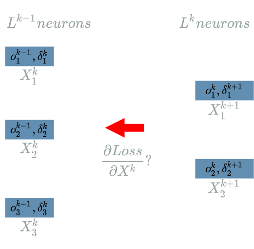
We are currently focusing on the $ L^{k} $ $ layer $, trying to compute:

\[\delta^{k} = \frac{\partial Loss}{\partial X^{k}}(o^{k-1})\]

In the backward pass article, we would use the chain rule in order to compute the explicit formula for $ \frac{\partial Loss}{\partial X^{k}} $.

We will see how to obtain this $ \delta^{k} $ with a more straight forward approach.

The principal idea is to go back to the very structure of $ L^{k} $ in order to find the impacts of $ X^{k} $ on the $ Loss $ function, knowing that the “future” learning flow has already been computed (by definition of the backward pass).

The structure for the $ L^{k} $ $ layer $ is:

• 2 output neurons
• 3 input neurons.

$ \delta^{k+1}_1 $ and $ \delta^{k+1}_2 $ are the “future” learning flow, we must back propagate the learning flow to $ \delta^{k}_1 $, $ \delta^{k}_2 $ and $ \delta^{k}_3 $.

Computing $ \delta^{k}_1 $

\[\delta^{k}_1 = \frac{\partial Loss}{\partial X^{k}_1}(o^{k-1}_1)\]

The interesting variable is $ X^{k}_1 $. Let us find its impacts on the $ Loss $ function. In fact, every output of $ L^{k} $ uses $ X^{k}_1 $. Indeed we can take a look at the two diagrams here to see that $ X^{k+1}_1 $ is linked to $ X^{k}_1 $ and that $ X^{k+1}_2 $ is also linked to $ X^{k}_1 $.

We have already seen examples (backward pass and batch learning) with multiple impacts: in the end we just added them all together.

We are now able to build the paths of impacts from $ X^{k}_1 $ to the $ Loss $ function.

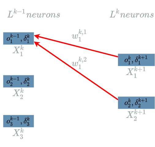
• $ X^{k}_1 $ impacts $ L^{k}_1 $ (definition of $ L^{k} $) which impacts the $ Loss $ function (“future” learning flow)
• $ X^{k}_1 $ impacts $ L^{k}_2 $ (definition of $ L^{k} $) which impacts the $ Loss $ function (“future” learning flow)

We add these 2 impacts, using the chain rule, to obtain the “impact formula”:

\[\delta^{k}_1 = \delta^{k+1}_1 . \frac{\partial L^{k}_1}{X^{k}_1}(o^{k-1}_1) + \delta^{k+1}_2 . \frac{\partial L^{k}_2}{X^{k}_1}(o^{k-1}_1)\]

We just have to compute:

\[\begin{align} \frac{\partial L^{k}_1}{\partial X^{k}_1} &= \frac{\partial (W^{k, 1}_1 . X^{k}_1 + W^{k, 1}_2 . X^{k}_2 + W^{k, 1}_3 . X^{k}_3 + B^{k}_1)}{\partial X^{k}_1} \\ &= W^{k, 1}_1 \end{align}\]

Then we evaluate this function on the values that have produced the final $ loss $:

\[\frac{\partial L^{k}_1}{X^{k}_1}(o^{k-1}_1) = w^{k, 1}_1\]

We do the same to obtain:

\[\frac{\partial L^{k}_2}{X^{k}_1}(o^{k-1}_1) = w^{k, 2}_1\]

We finally assemble these two results in the “impact formula”:

\[\boxed{\delta^{k}_1 = \delta^{k+1}_1 . w^{k, 1}_1 + \delta^{k+1}_2 . w^{k, 2}_1}\]

Computing $ \delta^{k}_2 $

\[\delta^{k}_2 = \frac{\partial Loss}{\partial X^{k}_2}(o^{k-1}_2)\]

The interesting variable is $ X^{k}_2 $. As in the previous paragraph, every output of $ L^{k} $ uses $ X^{k}_2 $. Indeed we can take a look at the last two diagrams here to see that $ X^{k+1}_1 $ is linked to $ X^{k}_2 $ and that $ X^{k+1}_2 $ is also linked to $ X^{k}_2 $.

We are now able to build the paths of impacts from $ X^{k}_2 $ to the $ Loss $ function.

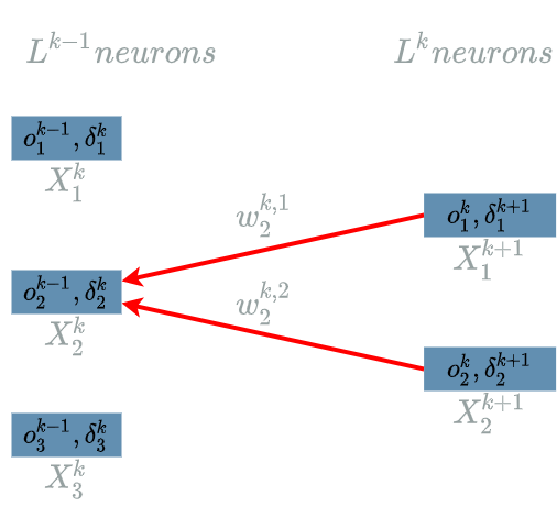
• $ X^{k}_2 $ impacts $ L^{k}_1 $ which impacts the $ Loss $ function
• $ X^{k}_2 $ impacts $ L^{k}_2 $ which impacts the $ Loss $ function

We add these 2 impacts, using the chain rule, to obtain the “impact formula”:

\[\delta^{k}_2 = \delta^{k+1}_1 . \frac{\partial L^{k}_1}{X^{k}_2}(o^{k-1}_2) + \delta^{k+1}_2 . \frac{\partial L^{k}_2}{X^{k}_2}(o^{k-1}_2)\]

We just have to compute:

\[\begin{align} \frac{\partial L^{k}_1}{\partial X^{k}_2} &= \frac{\partial (W^{k, 1}_1 . X^{k}_1 + W^{k, 1}_2 . X^{k}_2 + W^{k, 1}_3 . X^{k}_3 + B^{k}_1)}{\partial X^{k}_2} \\ &= W^{k, 1}_2 \end{align}\]

Then we evaluate this function on the values that have produced the final $ loss $:

\[\frac{\partial L^{k}_1}{X^{k}_2}(o^{k-1}_2) = w^{k, 1}_2\]

We do the same to obtain:

\[\frac{\partial L^{k}_2}{X^{k}_2}(o^{k-1}_2) = w^{k, 2}_2\]

We finally assemble these two results in the “impact formula”:

\[\boxed{\delta^{k}_2 = \delta^{k+1}_1 . w^{k, 1}_2 + \delta^{k+1}_2 . w^{k, 2}_2}\]

Computing $ \delta^{k}_3 $

\[\delta^{k}_3 = \frac{\partial Loss}{\partial X^{k}_3}(o^{k-1}_3)\]

The interesting variable is $ X^{k}_3 $. As in the previous paragraph, every output of $ L^{k+1} $ uses $ X^{k}_3 $. Indeed we can take a look at the last two diagrams here to see that $ X^{k+1}_1 $ is linked to $ X^{k}_3 $ and that $ X^{k+1}_2 $ is also linked to $ X^{k}_3 $.

We are now able to build the paths of impacts from $ X^{k}_3 $ to the $ Loss $ function.

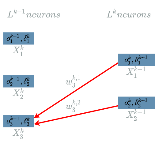
• $ X^{k}_3 $ impacts $ L^{k}_1 $ which impacts the $ Loss $ function
• $ X^{k}_3 $ impacts $ L^{k}_2 $ which impacts the $ Loss $ function

We add these 2 impacts, using the chain rule, to obtain the “impact formula”:

\[\delta^{k}_3 = \delta^{k+1}_1 . \frac{\partial L^{k}_1}{X^{k}_3}(o^{k-1}_3) + \delta^{k+1}_2 . \frac{\partial L^{k}_2}{X^{k}_3}(o^{k-1}_3)\]

We just have to compute:

\[\begin{align} \frac{\partial L^{k}_1}{\partial X^{k}_3} &= \frac{\partial (W^{k, 1}_1 . X^{k}_1 + W^{k, 1}_2 . X^{k}_2 + W^{k, 1}_3 . X^{k}_3 + B^{k}_1)}{\partial X^{k}_3} \\ &= W^{k, 1}_3 \end{align}\]

Then we evaluate this function on the values that have produced the final $ loss $:

\[\frac{\partial L^{k}_1}{X^{k}_3}(o^{k-1}_3) = w^{k, 1}_3\]

We do the same to obtain:

\[\frac{\partial L^{k}_2}{X^{k}_3}(o^{k-1}_3) = w^{k, 2}_3\]

We finally assemble these two results in the “impact formula”:

\[\boxed{\delta^{k}_3 = \delta^{k+1}_1 . w^{k, 1}_3 + \delta^{k+1}_2 . w^{k, 2}_3}\]

Backward Pass for the Weights

In this paragraph we continue focusing on the $ L^{k} $ $ layer $. This time we want to compute the opposite direction to follow for its weights’ update:

\[\delta w^{k} = \frac{\partial Loss}{\partial W}(o^{k-1})\]

We will use the exact same strategy as in the last paragraph. The principal idea is to go back to the very structure of $ L^{k} $ in order to find the impacts of $ W^{k} $ on the $ Loss $ function, knowing that the “future” learning flow has already been computed (by definition of the backward pass).

There are two more weights we have to update during the training phase: $ B^{k}_1 $ and $ B^{k}_2 $, the biases. Thus, we will have to compute $ \delta b^{k}_1 $ and $ \delta b^{k}_2 $.

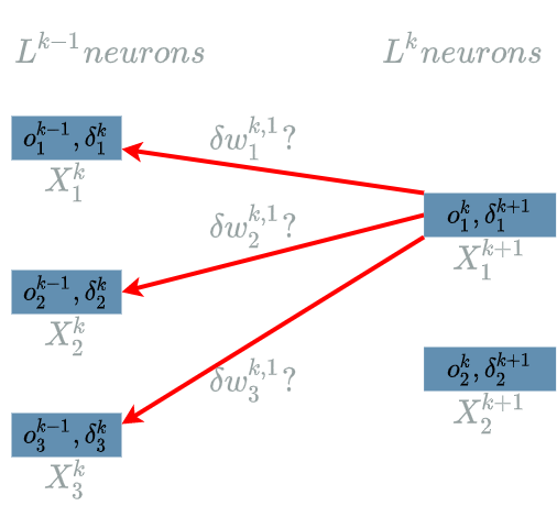
Computing $ \delta w^{k, 1}_1 $

\[\delta w^{k, 1}_1 = \frac{\partial Loss}{\partial W^{k, 1}_1}(o^{k-1}_1)\]

The interesting variable is $ W^{k, 1}_1 $. In the different diagrams it corresponds to $ w^{k, 1}_1 $, its value during the current backward pass. There is just one output of $ L^{k} $ that uses $ W^{k, 1}_1 $: $ L^{k}_1 $. Indeed we can take a look at the diagram here to see that $ o^{k}_1 $ is linked to $ w^{k, 1}_1 $.

We are now able to build the paths of impacts from $ W^{k, 1}_1 $ to the $ Loss $ function. This is in fact what we already saw in this diagram.

• $ W^{k, 1}_1 $ impacts $ L^{k}_1 $ which impacts the $ Loss $ function

We have only 1 impact, using the chain rule, we obtain the “impact formula”:

\[\delta w^{k, 1}_1 = \delta^{k+1}_1 . \frac{\partial L^{k}_1}{W^{k, 1}_1}(o^{k-1}_1)\]

We just have to compute:

\[\begin{align} \frac{\partial L^{k}_1}{\partial W^{k, 1}_1} &= \frac{\partial (W^{k, 1}_1 . X^{k}_1 + W^{k, 1}_2 . X^{k}_2 + W^{k, 1}_3 . X^{k}_3 + B^{k}_1)}{\partial W^{k, 1}_1} \\ &= X^{k}_1 \end{align}\]

Then we evaluate this function on the values that have produced the final $ loss $:

\[\frac{\partial L^{k}_1}{W^{k, 1}_1}(o^{k-1}_1) = o^{k-1}_1\]

We finally use this result in the “impact formula”:

\[\boxed{\delta w^{k, 1}_1 = \delta^{k+1}_1 . o^{k-1}_1}\]

Computing $ \delta w^{k, 1}_2 $ and $ \delta w^{k, 1}_3 $

Same as in the previous paragraph. The results are:

\[\boxed{\delta w^{k, 1}_2 = \delta^{k+1}_1 . o^{k-1}_2}\] \[\boxed{\delta w^{k, 1}_3 = \delta^{k+1}_1 . o^{k-1}_3}\]

Computing $ \delta w^{k, 2}_1 $

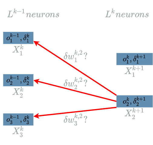
\[\delta w^{k, 2}_1 = \frac{\partial Loss}{\partial W^{k, 2}_1}(o^{k-1}_1)\]

The interesting variable is $ W^{k, 2}_1 $. In the different diagrams it corresponds to $ w^{k, 2}_1 $, its value during the current backward pass. There is just one output of $ L^{k} $ that uses $ W^{k, 2}_1 $: $ L^{k}_2 $. Indeed we can take a look at the diagram here to see that $ o^{k}_2 $ is linked to $ w^{k, 2}_1 $.

We are now able to build the paths of impacts from $ W^{k, 2}_1 $ to the $ Loss $ function. This is in fact what we already saw in this diagram.

• $ W^{k, 2}_1 $ impacts $ L^{k}_2 $ which impacts the $ Loss $ function

We have only 1 impact, using the chain rule, we obtain the “impact formula”:

\[\delta w^{k, 2}_1 = \delta^{k+1}_2 . \frac{\partial L^{k}_2}{W^{k, 2}_1}(o^{k-1}_1)\]

We just have to compute:

\[\begin{align} \frac{\partial L^{k}_2}{\partial W^{k, 2}_1} &= \frac{\partial (W^{k, 2}_1 . X^{k}_1 + W^{k, 2}_2 . X^{k}_2 + W^{k, 2}_3 . X^{k}_3 + B^{k}_2)}{\partial W^{k, 2}_1} \\ &= X^{k}_1 \end{align}\]

Then we evaluate this function on the values that have produced the final $ loss $:

\[\frac{\partial L^{k}_2}{W^{k, 2}_1}(o^{k-1}_1) = o^{k-1}_1\]

We finally use this result in the “impact formula”:

\[\boxed{\delta w^{k, 2}_1 = \delta^{k+1}_2 . o^{k-1}_1}\]

Computing $ \delta w^{k, 2}_2 $ and $ \delta w^{k, 2}_3 $

Same as in the previous paragraph. The results are:

\[\boxed{\delta w^{k, 2}_2 = \delta^{k+1}_2 . o^{k-1}_2}\] \[\boxed{\delta w^{k, 2}_3 = \delta^{k+1}_2 . o^{k-1}_3}\]

Computing $ \delta b^{k}_1 $

\[\delta b^{k}_1 = \frac{\partial Loss}{\partial B^{k}_1}(o^{k-1})\]

The interesting variable is $ B^{k}_1 $. There is just one output of $ L^{k} $ that uses $ B^{k}_1 $: $ L^{k}_1 $. This is clear when we take a take a look at the first equation of the forward pass paragraph.

We are now able to build the paths of impacts from $ B^{k}_1 $ to the $ Loss $ function.

• $ B^{k}_1 $ impacts $ L^{k}_1 $ which impacts the $ Loss $ function

We have only 1 impact, using the chain rule, we obtain the “impact formula”:

\[\delta b^{k}_1 = \delta^{k+1}_1 . \frac{\partial L^{k}_1}{\partial B^{k}_1}(o^{k-1})\]

We just have to compute:

\[\begin{align} \frac{\partial L^{k}_1}{\partial B^{k}_1} &= \frac{\partial (W^{k, 1}_1 . X^{k}_1 + W^{k, 1}_2 . X^{k}_2 + W^{k, 1}_3 . X^{k}_3 + B^{k}_1)}{\partial B^{k}_1} \\ &= 1 \end{align}\]

Then we evaluate this function on the values that have produced the final $ loss $:

\[\frac{\partial L^{k}_1}{\partial B^{k}_1}(o^{k-1}) = 1\]

We finally use this result in the “impact formula”:

\[\boxed{\delta b^{k}_1 = \delta^{k+1}_1}\]

Computing $ \delta b^{k}_2 $

\[\delta b^{k}_2 = \frac{\partial Loss}{\partial B^{k}_2}(o^{k-1})\]

The interesting variable is $ B^{k}_2 $. There is just one output of $ L^{k} $ that uses $ B^{k}_2 $: $ L^{k}_2 $. This is clear when we take a take a look at the second equation of the forward pass paragraph.

We are now able to build the paths of impacts from $ B^{k}_2 $ to the $ Loss $ function.

• $ B^{k}_2 $ impacts $ L^{k}_2 $ which impacts the $ Loss $ function

We have only 1 impact, using the chain rule, we obtain the “impact formula”:

\[\delta b^{k}_2 = \delta^{k+1}_2 . \frac{\partial L^{k}_2}{\partial B^{k}_2}(o^{k-1})\]

We just have to compute:

\[\begin{align} \frac{\partial L^{k}_2}{\partial B^{k}_2} &= \frac{\partial (W^{k, 2}_1 . X^{k}_1 + W^{k, 2}_2 . X^{k}_2 + W^{k, 2}_3 . X^{k}_3 + B^{k}_2)}{\partial B^{k}_2} \\ &= 1 \end{align}\]

Then we evaluate this function on the values that have produced the final $ loss $:

\[\frac{\partial L^{k}_2}{\partial B^{k}_2}(o^{k-1}) = 1\]

We finally use this result in the “impact formula”:

\[\boxed{\delta b^{k}_2 = \delta^{k+1}_2}\]

Example

We have already used a $ Linear $ $ layer $ in the “Example” of the previous articles. Let us have a look at the $ model $ we used in the weights article:

\[\begin{align} L1(X^1) &= X^1 & \text{ with } X^1 = (X^1_1, X^1_2, X^1_3) \\ L2(X^2, W^2) &= W^2 . X^2 & \text{ with } X^2 = (X^2_1, X^2_2, X^2_3) \\ & & \text{ and } W^2 = (W^2_1, W^2_2, W^2_3) \\ &= W^2_1 . X^2_1 + W^2_2 . X^2_2 + W^2_3 . X^2_3 \\ L3(X^3) &= X^3 \text{ if } X^3 \geq 0 \text{ else } 0 \\ \\ model(X) &= L3(L2(L1(X))) & \text{ with } X = (X_1, X_2, X_3) \\ Loss(X^4, Y^{truth}) &= \frac{1}{2} (X^4 - Y^{truth})^2 \end{align}\]

$ L2 $ is indeed a $ Linear $ $ layer $. It has two particularities compared to the neural structure we have seen here.

• It does not use any $ B^2 $ bias
• It has only 1 output neuron

Note that the 1 output neuron is something that is necessary for the very structure of the problem we are trying to solve in the “Example” (see the first article): from data input that have 3 numbers ((broccoli, Tagada strawberries, workout hours) => 3 neurons) we want to predict data output that is just one number ((good shape or not) => 1 neuron).

Let us recap the $ L2 $ neural structure:

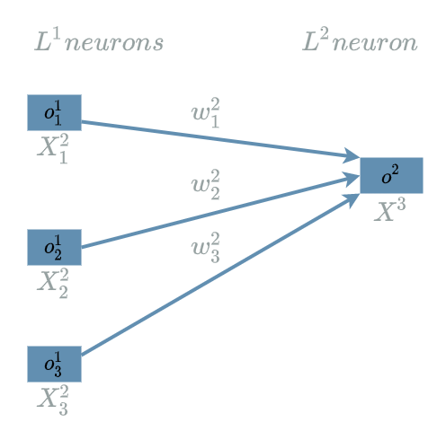
Forward Pass for L2

By definition, we just have to use the $ L2 $ explicit formula:

\[\begin{align} L2(X^2, W^2) &= W^2 . X^2 & \text{ with } X^2 = (X^2_1, X^2_2, X^2_3) \\ & & \text{ and } W^2 = (W^2_1, W^2_2, W^2_3) \\ &= W^2_1 . X^2_1 + W^2_2 . X^2_2 + W^2_3 . X^2_3 \\ \end{align}\]

The neural structure we have seen in the previous paragraph is another way to formalize the transformation of the $ L2 $ input values: $ o^1_1 $, $ o^1_2 $ and $ o^1_3 $ into the $ L2 $ output values: $ o^2 $. Still, it is more useful as a tool to find the impacts of the input neurons in order to compute the different elements of the backward pass.

Backward Pass for L2

We have already computed the different elements.

In the backward pass for the learning flow, we found:

\[\delta^{k}_1 = \delta^{k+1}_1 . w^{k, 1}_1 + \delta^{k+1}_2 . w^{k, 2}_1\] \[\delta^{k}_2 = \delta^{k+1}_1 . w^{k, 1}_2 + \delta^{k+1}_2 . w^{k, 2}_2\] \[\delta^{k}_3 = \delta^{k+1}_1 . w^{k, 1}_3 + \delta^{k+1}_2 . w^{k, 2}_3\]

We adjust these formula to the current neural structure:

\[\boxed{\delta^{2}_1 = \delta^{3} . w^{2}_1}\] \[\boxed{\delta^{2}_2 = \delta^{3} . w^{2}_2}\]

and

\[\boxed{\delta^{2}_3 = \delta^{3} . w^{2}_3}\]

We summarize them as:

\[\delta^{2} = \delta^{3} . w^2\]

which is what we already computed in the backward pass article.

In the backward pass for the weights, we found:

\[\delta w^{k, 1}_1 = \delta^{k+1}_1 . o^{k-1}_1\] \[\delta w^{k, 1}_2 = \delta^{k+1}_1 . o^{k-1}_2\] \[\delta w^{k, 1}_3 = \delta^{k+1}_1 . o^{k-1}_3\]

In fact, we computed 6 formula for the weights and 2 formula for the biases. Considering the current neural structure it is clear we do not need the 3 last formula for the weights nor the formula for the biases. We just have to adapt the first 3 formula:

\[\boxed{\delta w^{2}_1 = \delta^{3} . o^1_1}\] \[\boxed{\delta w^{2}_2 = \delta^{3} . o^1_2}\] \[\boxed{\delta w^{2}_3 = \delta^{3} . o^1_3}\]

which we summarize as:

\[\delta w^{2} = \delta^{3} . o^1\]

Once more, we recognize the formula we found in the weights article.

Conclusion

We have explored the $ Linear $ $ layer $ and found out we already used this $ layer $ in the “Example” introduced in the second article.

We saw how the neural structure helps finding the impacts of the different neurons on the $ Loss $ function. This is the core of the backward pass and more generally the core of the learning process.

In the next article we will continue exploring the other $ layers $ of our “Example”.