Normalization Layer

Introduction

In the batch learning article, we saw a method that helps stabilizing the learning process. It is a global method that modifies the behavior of the gradient descent algorithm itself.

In this article we will discuss a much more localised method: applying normalization on the $ layer $ scope.

The Formula

The idea is that instead of considering one global methodology that “stabilizes” gradients, we will include a specific operation in some $ layers $ of our deep learning $ model $ in order to “stabilize” the output neurons ot these specific chosen $ layers $.

First of all, how should we “stabilize” the output neurons ?

In order to “stabilize”, we will compute a “norm”, representing the typical average output of the neurons of our chosen $ layer $. Let us note this $ mean $ value $ \mu $:

\[\mu = \frac{1}{\textbf{nb elements}} . \sum_{elem=0}^{\textbf{nb elements} - 1} o_{elem}\]

We also want to know about the typical difference we might observe between one output neuron of our considered $ layer $ and the $ mean $ above. This is called the standard deviation, noted $ \sigma $:

\[\sigma = \sqrt{\left[\frac{1}{\textbf{nb elements}} . \sum_{elem=0}^{\textbf{nb elements} - 1} (o_{elem} - \mu)^2\right] + \epsilon}\]

with \(\epsilon \approx 0\).

The Shapes of Normalization

We have the two principal elements needed to “stabilize” the output neurons of one $ layer $. But there is still an important problem to solve…

In the linear function and the second dimension articles, we respectively saw how the $ Linear $ and the $ Convolution $ $ layers $ build representations.

For the $ Linear $ $ layer $, the “meaning” is hold by each of the output neurons themselves. For the $ Convolution $ $ layer $, the “meaning” is hold by the different channels, composed of output neurons organized in a grid.

During the normalization process we will have to preserve these “meaning” intact, avoiding to mix output neurons that do not represent “the same thing”.

The Linear Layer

Let us suppose $ L^{k-1} $ is a $ Linear $ $ layer $ that produces 3 output neurons. We want to compute its “norm” elements as in the previous paragraph.

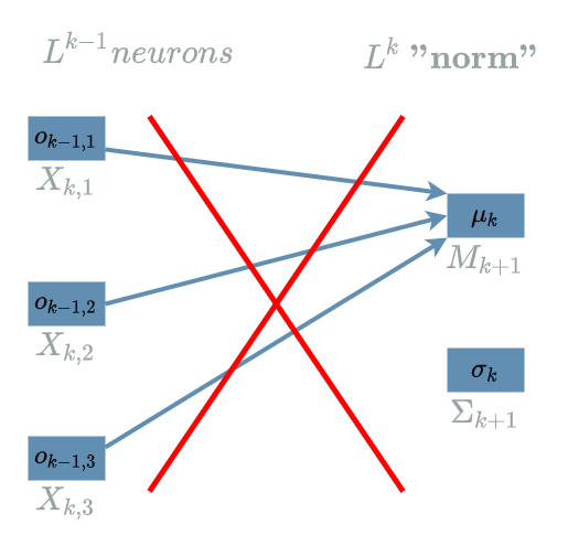
In the diagram above, we are computing the “norm” elements mixing different output neurons which is a bad idea.

In order to cope with this problem, we are going to use the idea of the batch learning article and compute the “norm” elements thanks to output neurons that are in the same “meaning” but different batch.

In the diagram below, we have drawn the same $ layer $ as before but for a batch size of 3.

The Convolution Layer

Let us suppose $ L^{k-1} $ is a $ Convolution $ $ layer $ that produces 3 output channels of a certain size $ (width, height) $. We want to compute its “norm” elements as in the previous paragraph.

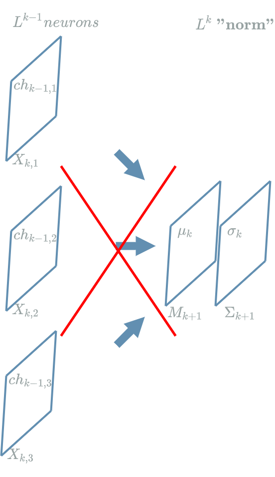
In the diagram above, the proposition was to compute the “norm” elements on each “pixel” so that:

\[\begin{align} \mu_{k,0,0} &= & \frac{1}{3} . (ch_{k-1,1,0,0} + ch_{k-1,2,0,0} + ch_{k-1,3,0,0}) \\ \sigma_{k,0,0} &= & \sqrt{\frac{1}{3} . \left[(ch_{k-1,1,0,0} - \mu_{k,0,0})^2 + (ch_{k-1,2,0,0} - \mu_{k,0,0})^2 + (ch_{k-1,3,0,0} - \mu_{k,0,0})^2\right] + \epsilon} \end{align}\]

Once more, we have the same problem as in the previous paragraph: we are computing the “norm” elements mixing output neurons of different channels.

In order to cope with this problem, we may use the same idea as before but there is a more interesting move to do here

Indeed, as each of our channels is made of multiple neurons, the “pixels”, we may use these different “pixels” to compute the “norm” elements for each channel. That way, we are not mixing neurons from different channels together.

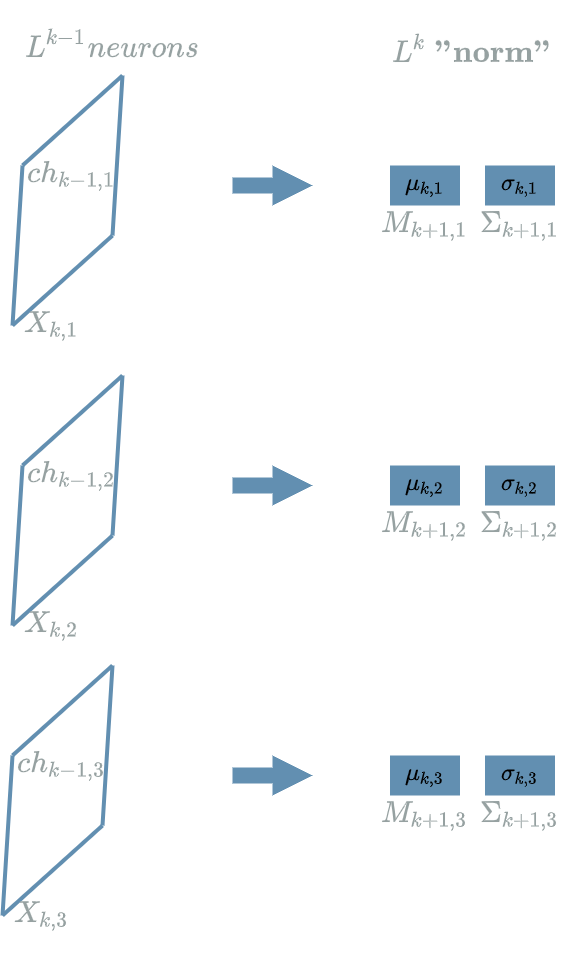
In the diagram above, the proposition was to compute the “norm” elements on each channel so that:

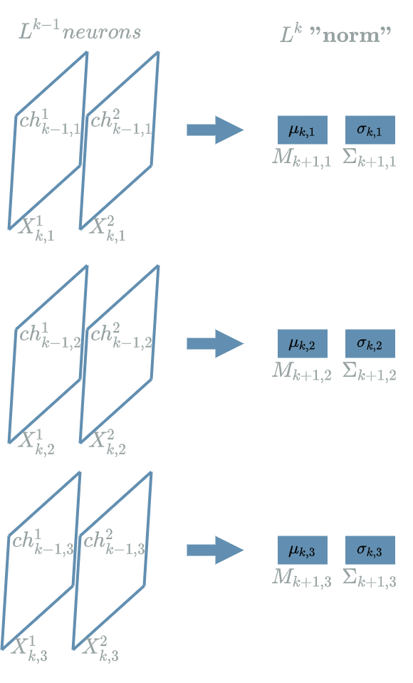
\[\begin{align} \mu_{k,1} &= & \frac{1}{width . height} . (ch_{k-1,1,0,0} + ... + ch_{k-1,1,0,width-1} \\ & & + ... \\ & & + ch_{k-1,1,height-1,0} + ... + ch_{k-1,1,height-1,width-1}) \\ \sigma_{k,1,tmp}^2 &= & (ch_{k-1,1,0,0} - \mu_{k,1})^2 + ... + (ch_{k-1,1,0,width-1} - \mu_{k,1})^2 \\ & & + ... \\ & & + (ch_{k-1,1,height-1,0} - \mu_{k,1})^2 + ... + (ch_{k-1,1,height-1,width-1} - \mu_{k,1})^2 \\ \sigma_{k,1} &= & \sqrt{\frac{1}{width . height} . \sigma_{k,1,tmp}^2 + \epsilon} \end{align}\]

Finally, the method used in the previous paragraph also applies in a batch learning setting. In the diagram below, we have drawn the same $ layer $ as before but for a batch size of 2.

Forward Pass

From now on we will make the assumption we have already chosen the good shape for normalization as mentioned in the previous paragraph: let us suppose that we are looking at 3 elements that do not mix different output neurons. These 3 elements may be the 3 batches of one output neuron of a $ Linear $ $ layer $ or the 3 batches of one really small channel of size (1,1) in a $ Convolution $ $ layer $.

We already know how to compute the “norm” elements for these 3 elements, noted $ o^1{k-1} $, $ o^2{k-1} $ and $ o^3_{k-1} $:

\[\begin{align} \mu_k &= & \frac{1}{3} . (o^1_{k-1} + o^2_{k-1} + o^3_{k-1}) \\ \sigma_k &= & \sqrt{\frac{1}{3} . \left[(o^1_{k-1} - \mu_k)^2 + (o^2_{k-1} - \mu_k)^2 + (o^3_{k-1} - \mu_k)^2\right] + \epsilon} \end{align}\]

The question is now: how do we use these “norm” elements in order to build the “normalized” output neurons of our $ L^{k} $ $ Normalization $ layer $.

We are going to transform each of these output neurons so that the new average output and standard deviation for these elements are “compensated” by the “norm” elements computed before:

\[\begin{align} o^1_{k'} &= & \frac{o^1_{k-1} - \mu_k}{\sigma_k} \\ o^2_{k'} &= & \frac{o^2_{k-1} - \mu_k}{\sigma_k} \\ o^3_{k'} &= & \frac{o^3_{k-1} - \mu_k}{\sigma_k} \end{align}\]

Let us note \(X^1_{(k+1)'}\), \(X^2_{(k+1)'}\) and \(X^3_{(k+1)'}\) the variables associated to the values \(o^1_{k'}\), \(o^2_{k'}\) and \(o^3_{k'}\).

The New “Norm” Elements

We have transformed our neurons \(o^1_{k-1}\), \(o^2_{k-1}\) and \(o^3_{k-1}\) of “norm” elements (\(\mu_k\), \(\sigma_k\) ) into \(o^1_{k'}\), \(o^2_{k'}\) and \(o^3_{k'}\) of “norm” elements (\(\mu_{k'}\), \(\sigma_{k'}\) ). Let us compute these new “norm” elements.

\[\begin{align} \mu_{k'} &= & \frac{1}{3} . (o^1_{k'} + o^2_{k'} + o^3_{k'}) \tag{1}\label{eq:mu_1} \\ &= & \frac{1}{3} . (\frac{o^1_{k-1} - \mu_k}{\sigma_k} + \frac{o^2_{k-1} - \mu_k}{\sigma_k} + \frac{o^3_{k-1} - \mu_k}{\sigma_k}) \tag{2}\label{eq:mu_2} \\ &= & \frac{1}{\sigma_k} . \left[\frac{1}{3} . (o^1_{k-1} + o^2_{k-1} + o^3_{k-1}) - \frac{1}{3} . 3\mu_k\right] \\ &= & \frac{1}{\sigma_k} . (\mu_k - \mu_k) \tag{3}\label{eq:mu_3} \\ &= & 0 \end{align}\]

\eqref{eq:mu_1}: definition of the average of \(o^1_{k'}\), \(o^2_{k'}\) and \(o^3_{k'}\).

\eqref{eq:mu_2}: definition of \(o^1_{k'}\), \(o^2_{k'}\) and \(o^3_{k'}\), see previous paragraph.

\eqref{eq:mu_3}: definition of the average of \(o^1_{k-1}\), \(o^2_{k-1}\) and \(o^3_{k-1}\).

\[\begin{align} \sigma_{k'} &= & \sqrt{\frac{1}{3} . \left[(o^1_{k'} - \mu_{k'})^2 + (o^2_{k'} - \mu_{k'})^2 + (o^3_{k'} - \mu_{k'})^2\right] + \epsilon} \tag{4}\label{eq:sigma_1} \\ &= & \sqrt{\frac{1}{3} . \left[(o^1_{k'})^2 + (o^2_{k'})^2 + (o^3_{k'})^2\right] + \epsilon} \tag{5}\label{eq:sigma_2} \\ &= & \sqrt{\frac{1}{3} . \left[(\frac{o^1_{k-1} - \mu_k}{\sigma_k})^2 + (\frac{o^2_{k-1} - \mu_k}{\sigma_k})^2 + (\frac{o^3_{k-1} - \mu_k}{\sigma_k})^2\right] + \epsilon} \tag{6}\label{eq:sigma_3} \\ &= & \frac{1}{\sigma_k} . \sqrt{\frac{1}{3} . \left[(o^1_{k-1} - \mu_k)^2 + (o^2_{k-1} - \mu_k)^2 + (o^3_{k-1} - \mu_k)^2\right] + \epsilon . (\sigma_k)^2} \\ &\approx & \frac{1}{\sigma_k} . \sigma_k \tag{7}\label{eq:sigma_4} \\ &\approx & 1 \end{align}\]

\eqref{eq:sigma_1}: definition of the standard deviation of \(o^1_{k'}\), \(o^2_{k'}\) and \(o^3_{k'}\).

\eqref{eq:sigma_2}: we already computed that \(\mu_{k'} = 0\).

\eqref{eq:sigma_3}: definition of \(o^1_{k'}\), \(o^2_{k'}\) and \(o^3_{k'}\), see previous paragraph.

\eqref{eq:sigma_4}: definition of the standard deviation of \(o^1_{k-1}\), \(o^2_{k-1}\) and \(o^3_{k-1}\) with the assumption that \(\epsilon . (\sigma_k)^2\) is small.

The average and standard deviation of our new output neurons are respectively 0 and 1.

The Final Shift

We have transformed the output neurons from “norm” elements (\(\mu_k\), \(\sigma_k\)) to (0, 1).

We could stop the transformation here, but it would be forgetting that we can insert some magical deep learning move

What if the new “norm” elements do not represent what is best for our $ L^k $ ? What if we could find some new average and standard deviation that serve our $ model $ better ?

This is what we will fix with 2 weights \(\Gamma_{k+1}\) and \(B_{k+1}\):

• \(B_{k+1}\) variable of value \(\beta_k\), the new average
• \(\Gamma_{k+1}\) variable of value \(\gamma_k\), the new standard deviation

We have already spoken about weights in the weights article, these 2 weights will be modified during the training phase so that their modification better suits the $ model $’s needs.

The final transform is:

\[\begin{align} o^1_{k} &= & \beta_k + \gamma_k . o^1_{k'} \\ o^2_{k} &= & \beta_k + \gamma_k . o^2_{k'} \\ o^3_{k} &= & \beta_k + \gamma_k . o^3_{k'} \end{align}\]

Without doing any computation, the new “norm” elements of these final output neurons are (\(\beta\), \(\gamma\)).

Let us recap our $ L^k $ $ Normalization $ $ layer $.

Backward Pass for the Learning Flow

We will have to be very careful to compute the backward pass for the $ Normalization $ $ layer $ because as we saw in this diagram, we have several intermediate elements that are $ function $ of other elements. In order to compute the different impacts correctly, we have to follow the order of the backward pass once more.

First of all, let us see the different $ function $ that appear in the previous diagram:

• \(X^1_k\), \(X^2_k\), \(X^3_k\): these functions only depend on elements that come in a previous $ layer $. Computing their own back propagation would be the task of the \(L^{k-1}\) \(layer\), not the current \(L^k\) one.
• \(M_{k+1}\) clearly depends on \(X^1_k\), \(X^2_k\), \(X^3_k\).
• \(\Sigma_{k+1}\) depends on \(X^1_k\), \(X^2_k\), \(X^3_k\) and \(M_{k+1}\).
• \(X^1_{k+1}\), \(X^2_{k+1}\), \(X^3_{k+1}\) depend on \(X^1_k\), \(X^2_k\), \(X^3_k\), \(M_{k+1}\), \(\Sigma_{k+1}\), \(B_{k+1}\) and \(\Gamma_{k+1}\).
• \(\Gamma_{k+1}\), \(B_{k+1}\) hopefully do not depend on anything, they will be updated in a later paragraph.

Thus, in order to take into account the different impacts, we have to compute our learning flow in the following order:

1. \(\delta X^1_{k+1}\), \(\delta X^2_{k+1}\), \(\delta X^3_{k+1}\) are given by construction of the backward pass (considering we are looking to back propagate the layer $ L^k $).
2. $ \delta \Sigma_{k+1} $
3. $ \delta M_{k+1} $
4. \(\delta X^1_k\), \(\delta X^2_k\), \(\delta X^3_k\)

mathematically shy people should jump to the conlusion

\(\delta \Sigma_{k+1}\)

As we can see in this diagram, the functions that depend on $ \Sigma_{k+1} $ are: \(X^1_{k+1}\), \(X^2_{k+1}\), \(X^3_{k+1}\). Said differently, $ \Sigma_{k+1} $ impacts: \(X^1_{k+1}\), \(X^2_{k+1}\) and \(X^3_{k+1}\).

We have computed several “impact formula” since the linear layer article, let us get straight to the point:

\[\delta \sigma_{k} = \delta^{k+1}_1 . \frac{\partial X^1_{k+1}}{\partial \Sigma_{k+1}}(.) + \delta^{k+1}_2 . \frac{\partial X^2_{k+1}}{\partial \Sigma_{k+1}}(.) + \delta^{k+1}_3 . \frac{\partial X^2_{k+1}}{\partial \Sigma_{k+1}}(.)\]

With:

\[\begin{align} \delta^{k+1}_1 &= & \frac{\partial Loss}{\partial X^{k+1}_1}(.) \\ \delta^{k+1}_2 &= & \frac{\partial Loss}{\partial X^{k+1}_2}(.) \\ \delta^{k+1}_3 &= & \frac{\partial Loss}{\partial X^{k+1}_3}(.) \end{align}\]

We put \((.)\) to remind ourselves we must evaluate the $ derivative $ $ function $. Yet, we hide the value where the $ function $ must be evaluated, see the linear layer article.

Let us compute \(\frac{\partial X^1_{k+1}}{\partial \Sigma_{k+1}}\):

\[\begin{align} \frac{\partial X^1_{k+1}}{\partial \Sigma_{k+1}} &= \frac{\partial (B_{k+1} + \Gamma_{k+1} . X^1_{(k+1)'})}{\partial \Sigma_{k+1}} \\ &= \frac{\partial (B_{k+1} + \Gamma_{k+1} . \frac{X^1_{k} - M_{k+1}}{\Sigma_{k+1}})}{\partial \Sigma_{k+1}} \tag{1}\label{eq:delta_sigma_1} \\ &= \Gamma_{k+1} . (X^1_{k} - M_{k+1}) . \frac{\partial (\frac{1}{\Sigma_{k+1}})}{\partial \Sigma_{k+1}} \\ &= \Gamma_{k+1} . (X^1_{k} - M_{k+1}) . \frac{-1}{(\Sigma_{k+1})^2} \\ &= -\frac{\Gamma_{k+1}}{\Sigma_{k+1}} . \frac{X^1_{k} - M_{k+1}}{\Sigma_{k+1}} \\ \frac{\partial X^1_{k+1}}{\partial \Sigma_{k+1}} &= - \frac{\Gamma_{k+1}}{\Sigma_{k+1}} . X^1_{(k+1)'} \tag{2}\label{eq:delta_sigma_2} \end{align}\]

\eqref{eq:delta_sigma_1}: definition of \(X^1_{(k+1)'}\), see the previous paragraph.

\eqref{eq:delta_sigma_2}: thanks again to the definition of \(X^1_{(k+1)'}\).

After having evaluated the previous $ derivative $ $ function $, we update the “impact formula”:

\[\boxed{\delta \sigma_{k} = - \frac{\gamma_k}{\sigma_k} . (\delta^{k+1}_1 . o^1_{k'} + \delta^{k+1}_2 . o^2_{k'} + \delta^{k+1}_3 . o^3_{k'})}\]

\(\delta M_{k+1}\)

As we can see in this diagram, $ M_{k+1} $ impacts \(X^1_{k+1}\), \(X^2_{k+1}\), \(X^3_{k+1}\) and \(\Sigma_{k+1}\).

We have the “impact formula”:

\[\delta \mu_{k} = \delta^{k+1}_1 . \frac{\partial X^1_{k+1}}{\partial M_{k+1}}(.) + \delta^{k+1}_2 . \frac{\partial X^2_{k+1}}{\partial M_{k+1}}(.) + \delta^{k+1}_3 . \frac{\partial X^2_{k+1}}{\partial M_{k+1}}(.) + \delta \sigma_{k} . \frac{\partial \Sigma_{k+1}}{\partial M_{k+1}}(.)\]

By construction of the backward pass we already know: \(\delta^{k+1}_1\), \(\delta^{k+1}_2\) and \(\delta^{k+1}_3\). Hopefully, we already computed \(\delta \sigma_{k}\) in the previous paragraph, thanks to the impact order !

Let us compute \(\frac{\partial X^1_{k+1}}{\partial M_{k+1}}\):

\[\begin{align} \frac{\partial X^1_{k+1}}{\partial M_{k+1}} &= \frac{\partial (B_{k+1} + \Gamma_{k+1} . X^1_{(k+1)'})}{\partial M_{k+1}} \\ &= \frac{\partial (B_{k+1} + \Gamma_{k+1} . \frac{X^1_{k} - M_{k+1}}{\Sigma_{k+1}})}{\partial M_{k+1}} \tag{1}\label{eq:delta_mu_1} \\ &= \Gamma_{k+1} . \frac{\partial (\frac{-M_{k+1}}{\Sigma_{k+1}})}{\partial M_{k+1}} \\ &= \Gamma_{k+1} . \frac{-1}{\Sigma_{k+1}} \\ \frac{\partial X^1_{k+1}}{\partial M_{k+1}} &= - \frac{\Gamma_{k+1}}{\Sigma_{k+1}} \end{align}\]

\eqref{eq:delta_mu_1}: definition of \(X^1_{(k+1)'}\), see the previous paragraph.

Let us also compute \(\frac{\partial \Sigma_{k+1}}{\partial M_{k+1}}\):

\[\begin{align} \frac{\partial \Sigma_{k+1}}{\partial M_{k+1}} &= \frac{\partial (\sqrt{\frac{1}{3} . \left[(X^1_{k} - M_{k+1})^2 + (X^2_{k} - M_{k+1})^2 + (X^3_{k} - M_{k+1})^2\right] + \epsilon})}{\partial M_{k+1}} \tag{2}\label{eq:delta_mu_2} \\ &= \frac{\frac{\partial (\frac{1}{3} . \left[(X^1_{k} - M_{k+1})^2 + (X^2_{k} - M_{k+1})^2 + (X^3_{k} - M_{k+1})^2\right] + \epsilon)}{\partial M_{k+1}}}{2 . \sqrt{\frac{1}{3} . \left[(X^1_{k} - M_{k+1})^2 + (X^2_{k} - M_{k+1})^2 + (X^3_{k} - M_{k+1})^2\right] + \epsilon}} \\ &= \frac{1}{2 . \Sigma_{k+1}} . \frac{\partial (\frac{1}{3} . \left[(X^1_{k} - M_{k+1})^2 + (X^2_{k} - M_{k+1})^2 + (X^3_{k} - M_{k+1})^2\right] + \epsilon)}{\partial M_{k+1}} \tag{3}\label{eq:delta_mu_3} \\ &= \frac{1}{2 . \Sigma_{k+1}} . \frac{1}{3} . \left[-2 . (X^1_{k} - M_{k+1}) - 2 . (X^2_{k} - M_{k+1}) - 2 . (X^3_{k} - M_{k+1})\right] \\ &= \frac{1}{2 . \Sigma_{k+1}} . \frac{1}{3} . (-2 * 3 * \frac{1}{3} . (X^1_{k} + X^2_{k} + X^3_{k}) + 2 * 3 . M_{k+1}) \\ &= \frac{1}{2 . \Sigma_{k+1}} . \frac{1}{3} . (-6 . M_{k+1} + 6 . M_{k+1}) \\ \frac{\partial \Sigma_{k+1}}{\partial M_{k+1}} &= 0 \end{align}\]

\eqref{eq:delta_mu_2}: definition of the standard deviation of \(X^1_k\), \(X^2_k\) and \(X^3_k\).

\eqref{eq:delta_mu_3}: thanks again to the definition of the standard deviation of \(X^1_k\), \(X^2_k\) and \(X^3_k\).

We update the “impact formula”:

\[\delta \mu_{k} = - \frac{\gamma_{k}}{\sigma_{k}} . (\delta^{k+1}_1 + \delta^{k+1}_2 + \delta^{k+1}_3) - \delta \sigma_{k} * 0\] \[\boxed{\delta \mu_{k} = - \frac{\gamma_{k}}{\sigma_{k}} . (\delta^{k+1}_1 + \delta^{k+1}_2 + \delta^{k+1}_3)}\]

\(\delta X^1_k\)

As we can see in this diagram, \(X^1_k\) impacts \(X^1_{k+1}\), \(M_{k+1}\) and \(\Sigma_{k+1}\).

We have the “impact formula”:

\[\delta^1_{k} = \delta^{k+1}_1 . \frac{\partial X^1_{k+1}}{\partial X^1_{k}}(.) + \delta \mu_{k} . \frac{\partial M_{k+1}}{\partial X^1_{k}}(.) + \delta \sigma_{k} . \frac{\partial \Sigma_{k+1}}{\partial X^1_{k}}(.)\]

By construction of the backward pass we already know: \(\delta^{k+1}_1\). In the previous 2 paragraphs we already computed: \(\delta \mu_{k}\) and \(\delta \sigma_{k}\).

Let us compute \(\frac{\partial X^1_{k+1}}{\partial X^1_{k}}\):

\[\begin{align} \frac{\partial X^1_{k+1}}{\partial X^1_{k}} &= \frac{\partial (B_{k+1} + \Gamma_{k+1} . X^1_{(k+1)'})}{\partial X^1_{k}} \\ &= \frac{\partial (B_{k+1} + \Gamma_{k+1} . \frac{X^1_{k} - M_{k+1}}{\Sigma_{k+1}})}{\partial X^1_{k}} \tag{1}\label{eq:delta_x_1} \\ \frac{\partial X^1_{k+1}}{\partial X^1_{k}} &= \frac{\Gamma_{k+1}}{\Sigma_{k+1}} \end{align}\]

\eqref{eq:delta_x_1}: definition of \(X^1_{(k+1)'}\), see the previous paragraph.

Let us compute \(\frac{\partial M_{k+1}}{\partial X^1_{k}}\):

\[\begin{align} \frac{\partial M_{k+1}}{\partial X^1_{k}} &= \frac{\partial (\frac{1}{3} . (X^1_{k} + X^2_{k} + X^3_{k}))}{\partial X^1_{k}} \tag{2}\label{eq:delta_x_2} \\ \frac{\partial M_{k+1}}{\partial X^1_{k}} &= \frac{1}{3} \end{align}\]

\eqref{eq:delta_x_2}: definition of the average of \(X^1_{k}\), \(X^2_{k}\) and \(X^3_{k}\).

Let us compute \(\frac{\partial \Sigma_{k+1}}{\partial X^1_{k}}\):

\[\begin{align} \frac{\partial \Sigma_{k+1}}{\partial X^1_{k}} &= \frac{\partial (\sqrt{\frac{1}{3} . \left[(X^1_{k} - M_{k+1})^2 + (X^2_{k} - M_{k+1})^2 + (X^3_{k} - M_{k+1})^2\right] + \epsilon})}{\partial X^1_{k}} \tag{3}\label{eq:delta_x_3} \\ &= \frac{\frac{\partial (\frac{1}{3} . \left[(X^1_{k} - M_{k+1})^2 + (X^2_{k} - M_{k+1})^2 + (X^3_{k} - M_{k+1})^2\right] + \epsilon)}{\partial X^1_{k}}}{2 . \sqrt{\frac{1}{3} . \left[(X^1_{k} - M_{k+1})^2 + (X^2_{k} - M_{k+1})^2 + (X^3_{k} - M_{k+1})^2\right] + \epsilon}} \\ &= \frac{1}{2 . \Sigma_{k+1}} . \frac{\partial (\frac{1}{3} . \left[(X^1_{k} - M_{k+1})^2 + (X^2_{k} - M_{k+1})^2 + (X^3_{k} - M_{k+1})^2\right] + \epsilon)}{\partial X^1_{k}} \tag{4}\label{eq:delta_x_4} \\ &= \frac{1}{2 . \Sigma_{k+1}} . \frac{1}{3} . \left[2 . (X^1_{k} - M_{k+1})\right] \\ &= \frac{1}{3} . \frac{X^1_{k} - M_{k+1}}{\Sigma_{k+1}} \\ \frac{\partial \Sigma_{k+1}}{\partial X^1_{k}} &= \frac{1}{3} . X^1_{(k+1)'} \tag{5}\label{eq:delta_x_5} \end{align}\]

\eqref{eq:delta_x_3}: definition of the standard deviation of \(X^1_k\), \(X^2_k\) and \(X^3_k\).

\eqref{eq:delta_x_4}: thanks again to the definition of the standard deviation of \(X^1_k\), \(X^2_k\) and \(X^3_k\).

\eqref{eq:delta_x_5}: definition of \(X^1_{(k+1)'}\), see the previous paragraph.

We update the “impact formula”:

\[\begin{align} \delta^1_{k} &= & \delta^{k+1}_1 . \frac{\gamma_k}{\sigma_k} \\ & & - \frac{\gamma_k}{\sigma_k} . (\delta^{k+1}_1 + \delta^{k+1}_2 + \delta^{k+1}_3) . \frac{1}{3} \\ & & - \frac{\gamma_k}{\sigma_k} . (\delta^{k+1}_1 . o^1_{k'} + \delta^{k+1}_2 . o^2_{k'} + \delta^{k+1}_3 . o^3_{k'}) . \frac{1}{3} . o^1_{k'} \end{align}\] \[\boxed{ \delta^1_{k} = \frac{\gamma_k}{\sigma_k} . \frac{1}{3} . \left[3 . \delta^{k+1}_1 - (\delta^{k+1}_1 + \delta^{k+1}_2 + \delta^{k+1}_3) - (\delta^{k+1}_1 . o^1_{k'} + \delta^{k+1}_2 . o^2_{k'} + \delta^{k+1}_3 . o^3_{k'}) . o^1_{k'}\right] }\]

The same logic allows to find:

\[\boxed{ \delta^2_{k} = \frac{\gamma_k}{\sigma_k} . \frac{1}{3} . \left[3 . \delta^{k+1}_2 - (\delta^{k+1}_1 + \delta^{k+1}_2 + \delta^{k+1}_3) - (\delta^{k+1}_1 . o^1_{k'} + \delta^{k+1}_2 . o^2_{k'} + \delta^{k+1}_3 . o^3_{k'}) . o^2_{k'}\right] }\] \[\boxed{ \delta^3_{k} = \frac{\gamma_k}{\sigma_k} . \frac{1}{3} . \left[3 . \delta^{k+1}_3 - (\delta^{k+1}_1 + \delta^{k+1}_2 + \delta^{k+1}_3) - (\delta^{k+1}_1 . o^1_{k'} + \delta^{k+1}_2 . o^2_{k'} + \delta^{k+1}_3 . o^3_{k'}) . o^3_{k'}\right] }\]

Backward Pass for the Weights

We have no more diagram here but the impacts of \(\Gamma_{k+1}\) and \(B_{k+1}\) are straight: \(X^1_{k+1}\), \(M_{k+1}\) and \(\Sigma_{k+1}\).

We have the “impact formulas”:

\[\delta \gamma_{k} = \delta^{k+1}_1 . \frac{\partial X^1_{k+1}}{\partial \Gamma_{k+1}}(.) + \delta^{k+1}_2 . \frac{\partial X^2_{k+1}}{\partial \Gamma_{k+1}}(.) + \delta^{k+1}_3 . \frac{\partial X^3_{k+1}}{\partial \Gamma_{k+1}}(.)\] \[\delta \beta_{k} = \delta^{k+1}_1 . \frac{\partial X^1_{k+1}}{\partial B_{k+1}}(.) + \delta^{k+1}_2 . \frac{\partial X^2_{k+1}}{\partial B_{k+1}}(.) + \delta^{k+1}_3 . \frac{\partial X^3_{k+1}}{\partial B_{k+1}}(.)\]

Let us compute \(\frac{\partial X^1_{k+1}}{\partial \Gamma_{k+1}}\):

\[\begin{align} \frac{\partial X^1_{k+1}}{\partial \Gamma_{k+1}} &= \frac{\partial (B_{k+1} + \Gamma_{k+1} . X^1_{(k+1)'})}{\partial \Gamma_{k+1}} \\ &= X^1_{(k+1)'} \\ \end{align}\]

Let us compute \(\frac{\partial X^1_{k+1}}{\partial B_{k+1}}\):

\[\begin{align} \frac{\partial X^1_{k+1}}{\partial B_{k+1}} &= \frac{\partial (B_{k+1} + \Gamma_{k+1} . X^1_{(k+1)'})}{\partial B_{k+1}} \\ &= 1 \\ \end{align}\]

We update the “impact formulas”:

\[\boxed{ \delta \gamma_{k} = \delta^{k+1}_1 . o^1_{k'} + \delta^{k+1}_2 . o^2_{k'} + \delta^{k+1}_3 . o^3_{k'} }\] \[\boxed{ \delta \beta_{k} = \delta^{k+1}_1 + \delta^{k+1}_2 + \delta^{k+1}_3 }\]

Conclusion

We have seen the normalization process can be run during the training phase at a precise place in the $ model $ thanks to the $ Normalization $ $ layer $. We saw that this $ layer $ implies some difficult computations during the backward pass.

In the next article we will use our $ layers $ in order to build a simple deep learning $ model $ and investigate our first deep learning task: classification !