Linear Function

Introduction

In the previous article, we illustrated the balance that occurs after each weights update of the gradient descent algorithm.

In this article we will investigate the purpose of the $ Linear $ network.

Note that a network and a $ model $ are very similar. We use the word network to refer to the general structure of the $ model $.

Also note that the simple $ model $ used so far (see the second article) is not linear in the mathematical sense because of the use of $ activation $ $ layers $ (which imply a non linearity, see the activation layer article). We call linear in the sense that the main learning $ layer $ is a $ Linear $ one (see the linear layer article).

From a Neuron Perspective

Let us go back to one situation we saw in the linear layer article. Let us consider one $ L^k $ $ Linear $ $ layer $ and suppose it has 2 output neurons: $ o^{k}_1 $ and $ o^{k}_2 $. Let us suppose $ L^{k-1} $ produces 3 output neurons: $ o^{k-1}_1 $, $ o^{k-1}_2 $ and $ o^{k-1}_3 $.

During the forward pass of $ L^k $ we expect to have the formulas:

\[\begin{align} o^{k}_1 &= w^{k, 1}_1 . o^{k-1}_1 + w^{k, 1}_2 . o^{k-1}_2 + w^{k, 1}_3 . o^{k-1}_3 + b^{k}_1 \\ o^{k}_2 &= w^{k, 2}_1 . o^{k-1}_1 + w^{k, 2}_2 . o^{k-1}_2 + w^{k, 2}_3 . o^{k-1}_3 + b^{k}_2 \end{align}\]

In this paragraph we want to illustrate the role of one neuron as an individual. For the moment we suppose that $ b^{k}_1 = 0 $ and $ b^{k}_2 = 0 $, our formulas become:

\[\begin{align} o^{k}_1 &= w^{k, 1}_1 . o^{k-1}_1 + w^{k, 1}_2 . o^{k-1}_2 + w^{k, 1}_3 . o^{k-1}_3 \\ o^{k}_2 &= w^{k, 2}_1 . o^{k-1}_1 + w^{k, 2}_2 . o^{k-1}_2 + w^{k, 2}_3 . o^{k-1}_3 \end{align}\]

Our main question here is: what makes $ o^{k}_1 $ and $ o^{k}_2 $ different ?

They both share the same immediate “data input”: $ o^{k-1}_1 $, $ o^{k-1}_2 $ and $ o^{k-1}_3 $. But they create different “meaning” of these “data input”: this “meaning” is what we called representation in the second article.

We immediately understand that what actually build the different representations are the weights. Thanks to the weights, the different output neurons will be differently correlated to the immediate “data input” of the previous $ L^{k-1} $ $ layer $.

For example, the weights for $ o^{k}_1 $ could be: $ w^{k, 1}_1 > 0 $, $ w^{k, 1}_2 < 0 $ and $ w^{k, 1}_3 > 0 $. Thanks to the $ o^{k}_1 $ formula above, this means that $ o^{k}_1 $ increases when the immediate “data input” $ o^{k-1} $ is $ (o^{k-1}_1 > 0, o^{k-1}_2 < 0, o^{k-1}_3 > 0) $.

To be more specific in the previous case:

locking $ o^{k-1}_2 $ and $ o^{k-1}_3 $ we have: $ o^{k-1}_1 $ ↑ => $ o^{k}_1 $ ↑ and $ o^{k-1}_1 $ ↓ => $ o^{k}_1 $ ↓
locking $ o^{k-1}_1 $ and $ o^{k-1}_3 $ we have: $ o^{k-1}_2 $ ↓ => $ o^{k}_1 $ ↑ and $ o^{k-1}_2 $ ↑ => $ o^{k}_1 $ ↓
locking $ o^{k-1}_1 $ and $ o^{k-1}_2 $ we have: $ o^{k-1}_3 $ ↑ => $ o^{k}_1 $ ↑ and $ o^{k-1}_3 $ ↓ => $ o^{k}_1 $ ↓

We can now artificially attribute a “meaning” to our different neurons. According to the special “meaning” attributed to $ o^{k-1} $, we can think about the “meaning” of $ o^{k}_1 $. For example, if $ o^{k-1} $ “means”: $ (\text{eat vegetables}, \text{ had a rare operation as a child}, \text{ workout regularly}) $, then the “meaning” of the $ o^k_1 $ output neuron could be: “be in good shape” because of the weights’ signs fixed earlier and the “logic” of the immediate “data input”.

In the same example, the weights for $ o^k_2 $ could be: $ w^{k, 2}_1 < 0 $, $ w^{k, 2}_2 = 0 $ and $ w^{k, 2}_3 < 0 $. In that way the “meaning” for the $ o^k_2 $ output neuron could be: “do not have a regular habit” because $ o^k_2 $ is linked negatively to $ o^{k-1}_1 $ (eat vegetables), $ o^{k-1}_3 $ (workout regularly) and not linked at all to $ o^{k-1}_2 $ (had a rare operation as a child).

What we must keep in mind here is that the weights give some sort of uniqueness to every neuron. It is then possible to give some “meaning” to the different neurons though that is the hardest part…

Link with the Activation Potential in Biology

In the previous paragraph, we saw the natural correlation linking the output neurons to the input neurons thanks to the weights of the $ Linear $ $ layer $.

Now we want to elaborate on the role of the $ activation $ $ layer $.

Let us take the same example where:

and:

$ w^{k, 1}_1 > 0 $, $ w^{k, 1}_2 < 0 $, $ w^{k, 1}_3 > 0 $
$ w^{k, 2}_1 < 0 $, $ w^{k, 2}_2 = 0 $, $ w^{k, 2}_3 < 0 $
$ o^{k-1} $ “means” $ (\text{eat vegetables}, \text{ had a rare operation as a child}, \text{ workout regularly}) $

For the sake of clarity, we will only discuss the $ o^{k}_1 $ case in the next paragraphs. The logic for $ o^k_2 $ is the same…

Looking back at $ o^{k}_1 $ we have:

locking $ o^{k-1}_2 $ and $ o^{k-1}_3 $ we have: $ o^{k-1}_1 $ ↑ => $ o^{k}_1 $ ↑ and $ o^{k-1}_1 $ ↓ => $ o^{k}_1 $ ↓
locking $ o^{k-1}_1 $ and $ o^{k-1}_3 $ we have: $ o^{k-1}_2 $ ↓ => $ o^{k}_1 $ ↑ and $ o^{k-1}_2 $ ↑ => $ o^{k}_1 $ ↓
locking $ o^{k-1}_1 $ and $ o^{k-1}_2 $ we have: $ o^{k-1}_3 $ ↑ => $ o^{k}_1 $ ↑ and $ o^{k-1}_3 $ ↓ => $ o^{k}_1 $ ↓

What is the problem between these variations and the “meaning” of “be in good shape” attributed to $ o^{k}_1 $ ?

The problem is that we do not really know “how much” $ o^{k}_1 $ should increase to really consider the state “be in good shape” to be true. Similarly we do not not know “how much” $ o^{k}_1 $ should decrease in order to consider the state “be in bad shape” to be true…

This is where we will add two more ingredients to save the meal: the biases ($ b^{k}_1 $ and $ b^{k}_2 $) and an $ activation $ $ layer $.

The Biases

Let us simply add the biases back to our $ L^{k} $ $ Linear $ $ layer $:

These biases add a “shift” that is not linked to $ o^{k-1} $.

The Activation Layer

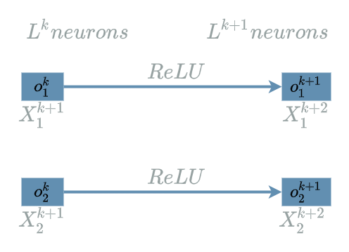
Let us also add an $ activation $ $ layer $ $ L^{k+1} $ right after $ L^{k} $ $ Linear $ $ layer $. $ L^k $ produces 2 output neurons. By definition of the $ activation $ $ layer $, $ L^{k+1} $ also produces 2 output neurons, each linked to one of the output neuron of $ L^{k} $. Let us also suppose that $ L^{k+1} $ uses the $ ReLU $ $ activation $ function:

Activation

The Biological Neuron

Let us recall the formula of the $ ReLU $ function:

\[ReLU(x) = \left\{\begin{align} x, & \text{ if $x \geq 0$}\\ 0, & \text{ otherwise} \end{align} \right.\]

What particularly interests us is the “filter” aspect of the $ ReLU $ $ activation $ function: everything under 0 is simply replaced by 0.

We are now able to modify the variations for $ o^{k}_1 $ and chain them to $ o^{k+1}_1 $:

locking $ o^{k-1}_2 $ and $ o^{k-1}_3 $ we have:
- $ o^{k-1}_1 $ ↑ => $ o^{k}_1 $ ↑ => $ o^{k+1}_1 > 0 $ on condition
- $ o^{k-1}_1 $ ↓ => $ o^{k}_1 $ ↓ => $ o^{k+1}_1 = 0 $ on condition
locking $ o^{k-1}_1 $ and $ o^{k-1}_3 $ we have:
- $ o^{k-1}_2 $ ↓ => $ o^{k}_1 $ ↑ => $ o^{k+1}_1 > 0 $ on condition
- $ o^{k-1}_2 $ ↑ => $ o^{k}_1 $ ↓ => $ o^{k+1}_1 = 0 $ on condition
locking $ o^{k-1}_1 $ and $ o^{k-1}_2 $ we have:
- $ o^{k-1}_3 $ ↑ => $ o^{k}_1 $ ↑ => $ o^{k+1}_1 > 0 $ on condition
- $ o^{k-1}_3 $ ↓ => $ o^{k}_1 $ ↓ => $ o^{k+1}_1 = 0 $ on condition

To see what the special condition is, we just have to wonder when we move from one “side” to the other. This special moment in the $ ReLU $ function happens at $ x = 0 $.

Let us look back at $ o^{k}_1 $:

\[o^{k}_1 = w^{k, 1}_1 . o^{k-1}_1 + w^{k, 1}_2 . o^{k-1}_2 + w^{k, 1}_3 . o^{k-1}_3 + b^{k}_1\]

We see that there is only one solution for $ o^{k}_1 = 0 $, it is when $ w^{k, 1}_1 . o^{k-1}_1 + w^{k, 1}_2 . o^{k-1}_2 + w^{k, 1}_3 . o^{k-1}_3 = - b^{k}_1 $.

This means that $ - b^{k}_1 $ is the threshold of our special condition:

when $ w^{k, 1}_1 . o^{k-1}_1 + w^{k, 1}_2 . o^{k-1}_2 + w^{k, 1}_3 . o^{k-1}_3 \leq - b^{k}_1 $ we have $ o^{k+1}_1 = 0 $
when $ w^{k, 1}_1 . o^{k-1}_1 + w^{k, 1}_2 . o^{k-1}_2 + w^{k, 1}_3 . o^{k-1}_3 > - b^{k}_1 $ we have $ o^{k+1}_1 > 0 $

Said differently, we now have a concrete threshold: $ - b^{k}_1 $ above which our $ o^{k+1}_1 $ neuron will be activated and let the signal pass. Under this threshold, the neuron will do nothing and block the signal.

In fact we have come from a “meaning” of “be in good shape” for $ o^k_1 $ to the exact same “meaning” for $ o^{k+1}_1 $. But the $ o^{k+1}_1 $ neuron looks like a biological neuron: it helps make a decision on a concrete physical impulse. This is the third reason of the use of $ activation $ $ layers $ we saw in the activation layer article.

While it seems interesting to mimic this “biological” neuron, we have already seen it may not be such a good idea in the previous article. The main problem being the backward pass. The good news is: our brain does not strictly rely on the backward pass…

Backward Pass

In this paragraph we want to illustrate the logic behind the backward pass for the $ Linear $ $ layer $.

We use the same $ layers $ as in the first paragraph:

$ L^{k-1} $ with 3 output neurons
$ L^k $ $ Linear $ $ layer $ with 2 output neurons

For the sake of clarity, we will focus on $ \delta^{k}_1 $ in the following:

Linear

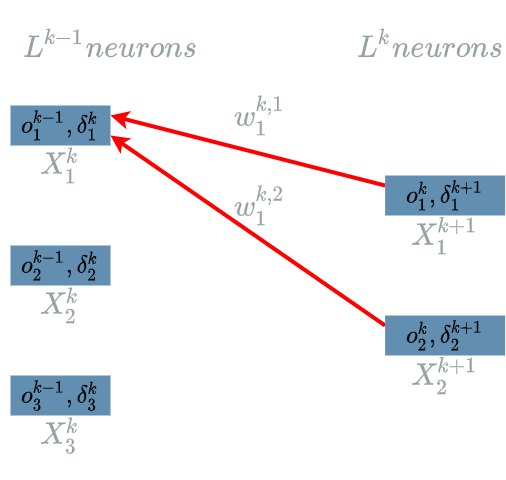
In the linear layer article, we already saw the formula for the retro propagation of the learning flow during the backward pass:

\[\boxed{\delta^{k}_1 = \delta^{k+1}_1 . w^{k, 1}_1 + \delta^{k+1}_2 . w^{k, 2}_1}\]

In the previous article, we saw how the backward pass preserves the “balance” in the learning flow. Let see how this logic applies on our $ Linear $ $ layer $.

Let us suppose $ \delta^{k+1}_1 < 0 $ and $ \delta^{k+1}_2 > 0 $. We know what this means:

a small increase in $ o^1_k $ would decrease the value of $ loss $ (which is actually our goal)
a small increase in $ o^2_k $ would increase the value of $ loss $ (which is the opposite of our goal)

We want to follow the current direction for $ o^1_k $ but take the opposite direction for $ o^2_k $. Using the “meaning” in our first paragraph, an interpretation is that:

the output neuron $ o^1_k $ “be in good shape” should be “more” used in this situation
the output neuron $ o^2_k $ “do not have a regular habit” should be “less” used in this situation

Although $ o^1_k $ and $ o^2_k $ are linked positively with $ o^{k-1}_1 $ ($ w^{k, 1}_1 > 0 $ and $ w^{k, 2}_1 > 0 $), it is the formula:

\[\delta^{k}_1 = \delta^{k+1}_1 . w^{k, 1}_1 + \delta^{k+1}_2 . w^{k, 2}_1\]

that will help decide whether $ o^{k-1}_1 $ should be “more” used ($ \delta^{k}_1 < 0 $) or “less” used ($ \delta^{k}_1 > 0 $) in the current situation defined by the data: (data input, data output).

Focusing on $ o^{k-1}_1 $ it is interesting to note that:

during the forward pass, $ o^k_1 $ and $ o^k_2 $ are linked to $ o^{k-1}_1 $ thanks to $ w^{k, 1}_1 $ and $ w^{k, 2}_1 $
during the backward pass, $ \delta^{k}_1 $ is linked to $ \delta^{k+1}_1 $ and $ \delta^{k+1}_2 $ thanks to $ w^{k, 1}_1 $ and $ w^{k, 2}_1 $

The Linear Function

It is now clear that the $ Linear $ $ layer $ establishes correlations between its input neurons and its output neurons.

Each output neuron being linked with every input neurons via specific weights, the different output neurons may be seen as different new representations/”meaning” of the input neurons.

In order to build more abstract representations, one idea is to simply add multiple $ Linear $ $ layers $ one after another, building a deep learning $ model $.

There are two problems in doing so:

we are building a $ model $ with many weights as every $ Linear $ $ layer $ neurons are linked to every neurons of their previous $ layer $ => it might be very long to run the gradient descent algorithm on such a $ model $
we would lose the comprehension of the inner $ layers $ of neurons

Finally it seems it is not that necessary to follow that path. Indeed, we already saw an example of use of a $ Linear $ $ layer $ during the previous articles and there are other fields where very simple $ models $ are the best option: clinical data. We might wonder why ?

The answer is that clinical data are in fact their own “final” representation. We do not really need to build abstraction of them as they are already structured in themselves. The remaining task being to find the correlations between the data input and the data output, perfect for one $ Linear $ $ layer $…

Conclusion

Is has been a long time since we have introduced our simple $ Linear $ $ model $. For some reasons, we are not yet ready to build very deep $ models $ and for the moment it does not seem that necessary as finding correlations is already the goal of the $ Linear $ $ layer $.

In the next article, we will discover a field where deep learning $ models $ are necessary