The Second Dimension
Introduction
In the previous article, we saw that $ Linear $ network are already good at finding correlations among structured data.
In this article we will explore a field where the data is not structured. What solution could we find in such a case ?
Computer Vision
The typical field where data is not structured is Computer Vision. In this field, we would like
machines to understand images and video the way humans do.
The main problem is that humans are already used to talk about images as representations (introduced in the second article, we talked about them more in the previous article).
For example when I see an image of another human, I tend to identify his/her main characteristics: the hair color, the eyes, the hands… And in fact each of these characteristics are some sort of representations. In my mind, I can play with these representations, comparing them for example: this human is taller than this one. In a way, I have a representation for the entire world and any image I will see will only refer to the representations I know. If I happen to interact with other senses, such as taste, I just have to enrich my visual representation knowing the taste and view refer to the same one.
But for a machine, we must build this whole from scratch…
The Visual Information Flow
The first difference we should highlight between Human Vision and Computer Vision is the information flow (see the second article).
In the human case the visual information flow is physical. It starts with light on our retina before being translated into neurons activations / non activations in our brain.
In the machine case, we will only work with numbers. The good news is that we just have to do some computations on those numbers to describe what happens. The bad news is that there will be so many computations that it will be difficult to fully grasp how representations are built. Hence, it is important to try and understand the different transformations of our information flow across the different $ layers $ of our $ model $: this is our goal for the next articles.
Before building deep learning $ models $, let us start by converting our images into numbers!
Images, what are they ?
An image is a grid of a certain size. An image of size $ (height, width) $ will contain $ height * width $ pixels. Each pixel is a mix of the three primary colors $ (red, green, blue) $.
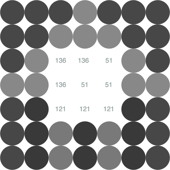
Let us imagine a very small image of size $ (7, 7) $ and zoom in so that we observe a house !
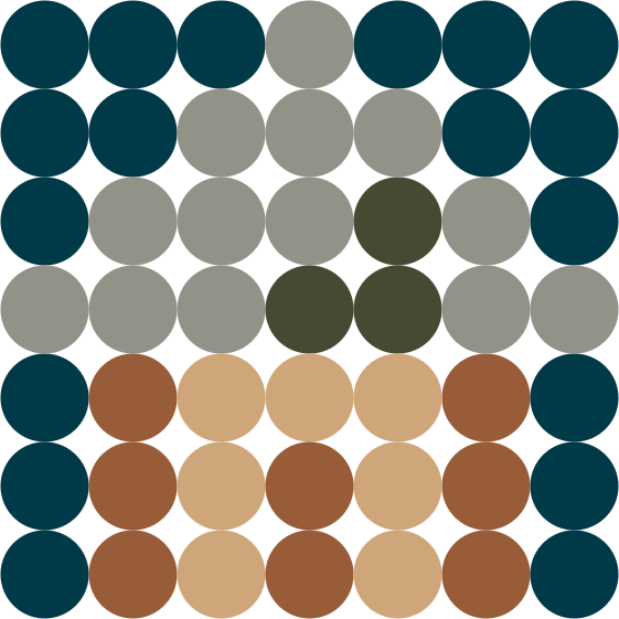
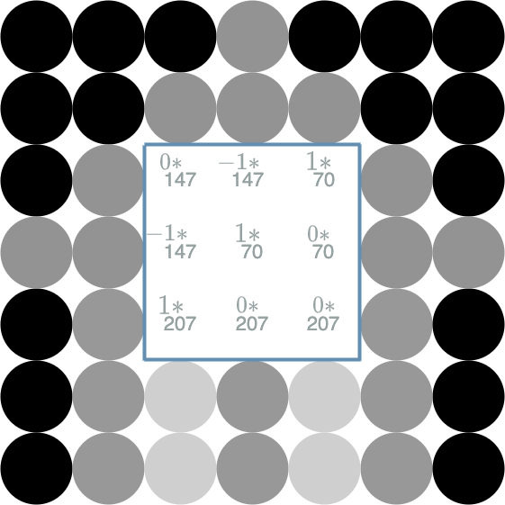
You may have guessed that each circle in this image actually represents a pixel of the image. As we mentioned in the previous paragraph, our brain is triggered by the light on different materials. But the same image can also be seen as the different numbers of the pixels. In the below image, I have hidden the center of the image to show some pixels’ values $ (red, green, blue) $.
Note that if the entire image was only numbers, you would have had no way of understanding the image as a house. This is why we have to build a system that allows the computer to “understand” those numbers.
Toward Visual Representations
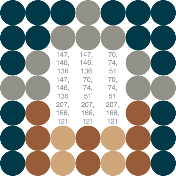
Here is the first operation to build our visual representations: instead of considering the grid of the previous numeric pixels, we will consider the three channels $ red $, $ green $ and $ blue $. The operation merely consists in splitting our grid of pixels into 3 channel grids of numbers.
We go from a grid of $ height * width $ pixels to 3 channel grids of $ height * width $ numbers.
Here is the the first channel grid ($ red $):
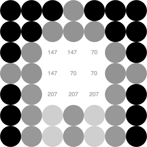
Here is the second channel grid ($ green $):
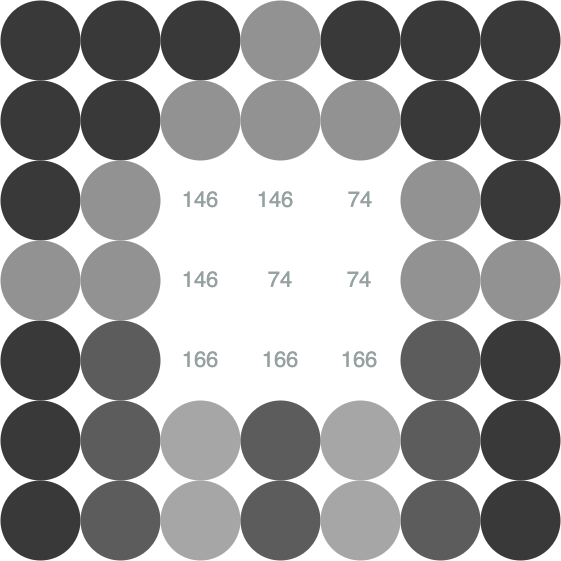
And here is the third channel grid ($ blue $):
We are now in the presence of 3 representations ! Here is how to go back to a real image: just stack the grid together to assemble the different numbers into pixels.
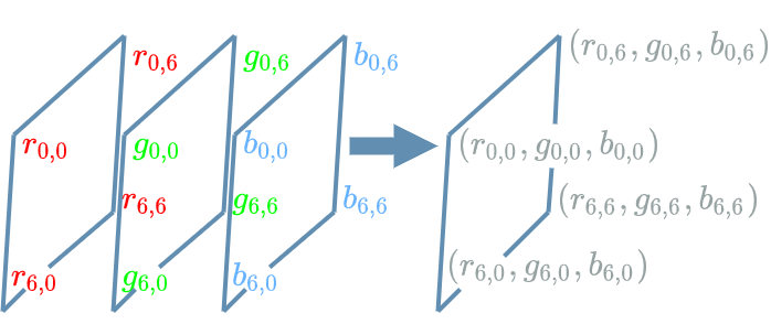
In the following I will speak about the “pixels” of the channels we introduced here. Keep in mind that these “pixels” are just one number at a precise position in a channel grid and not the pixels we talked about in the images paragraph.
Convolution Kernel
Working on images seems to complicate the structure of our data. Back to the first article, our data were vectors of numbers: example $ (100, 2000, 100) $. Dealing with images has increased the dimensionality of our data: from being 1 dimensional (a vector of numbers), they have become 2 dimensional (a vector of vector of numbers, or said differently a 2D array of numbers).
How can we process this new type of data ?
Let us introduce the convolution kernel: a new grid that will help us elaborate an operation on 2D arrays of numbers. The interesting part of this new grid is that it enables to capture spatial localisation particularities in the input channel (more on this in the example).
For now, let us take a small convolution kernel to fix the ideas:
\[\begin{bmatrix} 0 & -1 & 1 \\ -1 & 1 & 0 \\ 1 & 0 & 0 \end{bmatrix}\]We want to capture spatial localisation information on every “pixel” of the different channels of the previous paragraph. But first of all, how do we apply the kernel on just one “pixel” in a given channel ?
By taking the center of the kernel, aligning it on the “pixel” to process in the input channel and adding the different multiplied couples. The result is one “pixel” of the output channel.
Let us see how it works with the small kernel defined above:
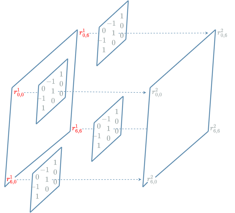
In the diagram above, only four new “pixels” are mentioned: \(r^2_{0,0}\), \(r^2_{6,0}\), \(r^2_{0,6}\) and \(r^2_{6,6}\). Please note that the kernel must be applied on EVERY “pixel” of the input channel in order to produce EVERY “pixel” of the output channel.
In order to be more specific, let us compute $ r^2_{6,0} $ for the red channel. An issue occurs: a part of the kernel does not cover the red grid, it covers an empty space. This is no big deal, we just replace the missing “pixels” by 0:
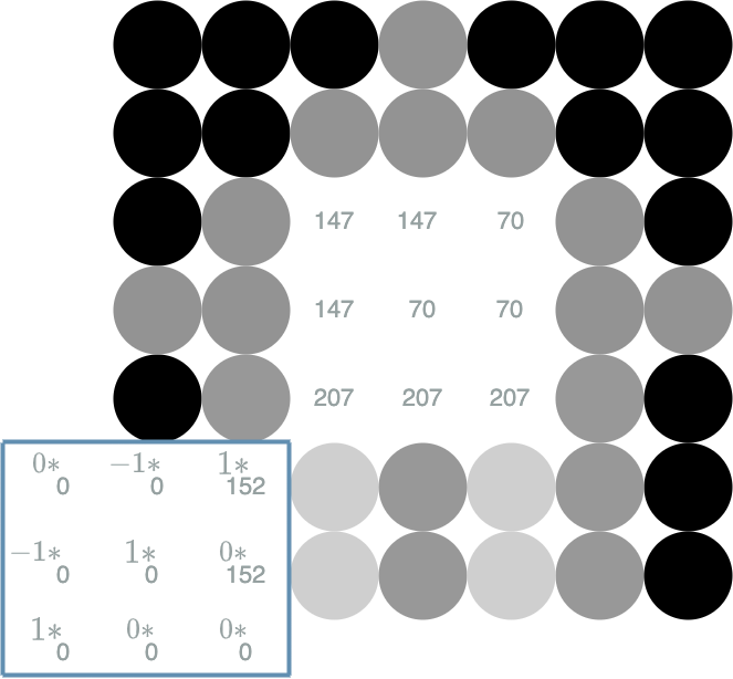
Then we add together the different multiplied couples:
\[\begin{align} r^2_{6,0} &= & (0 * 0) + (-1 * 0) + (1 * 152) \\ & & + (-1 * 0) + (1 * 0) + (0 * 152) \\ & & + (1 * 0) + (0 * 0) + (0 * 0) \\ r^2_{6,0} &= 152 & \end{align}\]Let us compute another example: $ r^2_{3, 3} $ for the red channel:
Convolution
We are now able to transform one input channel into one output channel thanks to some operation with a convolution kernel. But we must not lose our goal identified in the second article: elaborate $ layers $ that build abstract representations.
Let us go back to the linear function article. We took an example where $ L^k $ $ Linear $ $ layer $ had 3 input neurons and produced 2 output neurons. We noted a particular important fact:
“Each output neuron being linked with every input neurons via specific weights, the different output neurons may be seen as different new representations of the input neurons.”
We want to build representations the same way for our images. This means we need to preserve the combination power of our output neurons.
Let us suppose that we want to build only 1 new representation out of the 3 channels of the visual representations paragraph.
The solution is to attribute one convolution kernel for each and every one of the 3 input channels we have. Then, thanks to the previous paragraph, we know how to apply the particular kernel on the chosen channel in order to build a temporary (noted $ tmp $ below) new channel. We now have 3 temporary new channels that we can sum together (adding the “pixels” of the 3 temporary channels that are localized at the same place in the grid) in order to build the final new representation noted $ rep $ below.
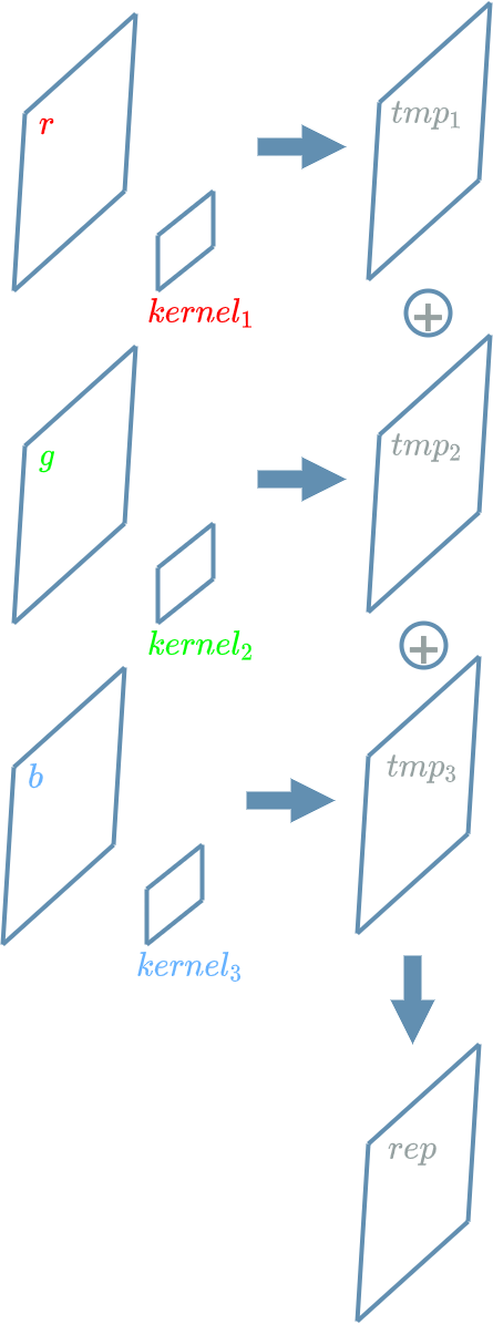
$ rep $ is a new representation that produces a new “meaning” thanks to the “meaning” of every input channels ($ r $, $ g $, $ b $).
Each time we want to build a new representation we have to use one specific convolution kernel for each input channel. This is very similar to what happened to the weights in the linear function article.
Small Experiment
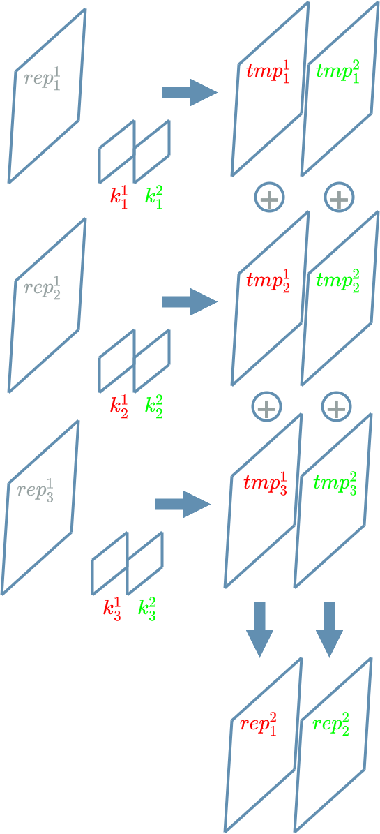
In this paragraph, we mimic the example where $ L^k $ $ Linear $ $ layer $ has 3 input neurons and produces 2 output neurons but this time with $ L^k $ $ Convolutional $ $ layer $.
$ L^k $ takes 3 channels as input and must produce 2 output channels. As we mentioned in the previous paragraph, for each output channel, we must choose one convolutional kernel for each input channel.
Now, let us add some meaning to these different channels. Let us suppose that:
- $ rep^1_1 $ represents “one eye”
- $ rep^1_2 $ represents “one nose”
- $ rep^1_3 $ represents “one mouth”.
As for the linear function article, we may build a “meaning” for $ rep^2_1 $ and $ rep^2_2 $. This “meaning” will directly depends on the previous channels’ meanings and their associated processing kernel.
Let us suppose that $ k^1_1 $, $ k^1_2 $ and $ k^1_3 $ are respectively:
\[\begin{bmatrix} 1 & 0 & 1 \\ 0 & 0 & 0 \\ 0 & 0 & 0 \end{bmatrix} \begin{bmatrix} 0 & 0 & 0 \\ 0 & 1 & 0 \\ 0 & 0 & 0 \end{bmatrix} \begin{bmatrix} 0 & 0 & 0 \\ 0 & 0 & 0 \\ 0 & 0 & 0 \end{bmatrix}\]As we apply $ k^1_1 $ on every “pixel” of the $ rep^1_1 $ channel “one eye”, we see that the maximum output “pixels” will be localised at input “pixels” that have the following neighbours:
- top left hand corner neighbour is “one eye”
- top right hand corner neighbour is “one eye”.
For $ k^1_2 $ and $ rep^1_2 $ “one nose”, the maximum output “pixels” will be localised at input “pixels” that are “one nose”.
For $ k^1_3 $ and $ rep^1_3 $ “one mouth”, there will be no maximum “pixels”, only 0.
Adding these 3 pieces together, the maximum output “pixels” will be localised at input “pixels” where the 3 convolution kernel are triggered at the same time by their associated channel. Here, this means that $ rep^2_1 $ represents the “top part of a face”.
Let us suppose that $ k^2_1 $, $ k^2_2 $ and $ k^2_3 $ are respectively:
\[\begin{bmatrix} 0 & 0 & 0 \\ 0 & 0 & 0 \\ 0 & 0 & 0 \end{bmatrix} \begin{bmatrix} 0 & 0 & 0 \\ 0 & 1 & 0 \\ 0 & 0 & 0 \end{bmatrix} \begin{bmatrix} 0 & 0 & 0 \\ 0 & 0 & 0 \\ 0 & 1 & 0 \end{bmatrix}\]For $ k^2_1 $ and $ rep^1_1 $ “one eye”, there will be no maximum “pixels”, only 0.
For $ k^2_2 $ and $ rep^1_2 $ “one nose”, the maximum output “pixels” will be localised at input “pixels” that are
“one nose”.
For $ k^2_3 $ and $ rep^1_3 $ “one mouth”, the maximum output “pixels” will be localised at input “pixels” that have the following neighbours:
- bottom neighbour is “one mouth”
If we add these 3 pieces together, we understand that $ rep^2_2 $ actually represents the “bottom part of a face”.
2D Representations
The two principal elements that allow the build of new representations in the 2D case are:
- the combination of previous representations (this is a legacy of the 1D case)
- the spatial context which is captured by the convolution kernels (this is specific to the 2D case)
We must keep in mind that one channel grid is an array of “pixels”. Each of these “pixels” being a number that has a particular “arbitrary meaning”. As we saw in the paragraph “The Biological Neuron” of the previous article, the number may indicate the presence of this “arbitrary meaning” according to some threshold: for example we may consider that above the threshold the “meaning” is right, below it is wrong.
In the previous paragraph, we had a channel
representing the “top part of a face”. There may be several different “pixels” where this information is right.
Same for the channel representing the “bottom part of a face”. Let us take a “pixel” and its neighbours.
In the case where the top neighbour of the “pixel” is a “top part of a face” (number is above a threshold) and
the bottom neighbour of the “pixel” is a “bottom part of a face” (number is also above a threshold, maybe not the same),
we understand that the “pixel” itself is a “whole face”.
This gives the hint that the representations are not really the grid themselves, but rather the vectors obtained when we stack the grids together:
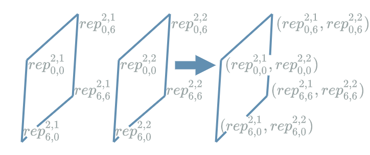
\((rep^{2,1}_{0,0}, rep^{2,2}_{0,0})\) is an example of such a vector. Note how similar it is to the method that allowed going from the representations to the real pixels in this diagram.
When we consider the grid of such vectors, we directly compare to the 1D case where our representations were vectors (see the linear function article). The sole difference being that in the 2D case our representations are placed in a grid because they have a 2D context…
Example
In this example, we will use the 3 input channels of the visual representations paragraph in order to better understand how the convolution kernels capture spatial localisation particularities and how they affect the representations.
Let us build a small convolutional model!
L1
The first layer is not the most interesting one: it plays the same role as the Input 1D described in the activation article. Here it is an Input 2D $ layer $ that just receives the 3 different channels of our house example.
L2
Much fun is happening now ![]()
This $ layer $ will be a $ Convolutional $ $ layer $. As we saw in the convolution paragraph, we must choose 3 different convolution kernels for each new channel built (because $ L1 $ $ layer $ has 3 output channels).
We want to build 6 new channels, this means that we need $ 3 * 6 = 18 $ different convolution kernels! For simplicity, we will suppose that the different convolution kernels are identical by group of 3 (the 3 convolution kernels used to produce first channel are identical, the 3 convolution kernels used to produce the second channel are identical…).
Here are the different convolution kernels that we will apply:
\[\begin{bmatrix} 0 & -1 & 1 \\ -1 & 1 & 0 \\ 1 & 0 & 0 \end{bmatrix} \begin{bmatrix} 1 & -1 & 0 \\ 0 & 1 & -1 \\ 0 & 0 & 1 \end{bmatrix}\] \[\begin{bmatrix} 1 & -1 & 1 \\ -1 & -1 & 1 \\ 1 & 1 & 1 \end{bmatrix}\] \[\begin{bmatrix} -1 & 1 & 1 \\ -1 & 1 & 1 \\ -1 & 1 & 1 \end{bmatrix} \begin{bmatrix} 1 & 1 & -1 \\ 1 & 1 & -1 \\ 1 & 1 & -1 \end{bmatrix}\] \[\begin{bmatrix} 1 & 1 & 1 \\ 1 & 1 & 1 \\ 1 & 1 & 1 \end{bmatrix}\]Spoiler alert:
- the first two kernels will be triggered by the house’s roof (note their structure in diagonal)
- the third kernel will detect the house’s window
- the following two kernels will detect the house’s walls (note their structure in vertical line)
- the last kernel will detect the inside of the house
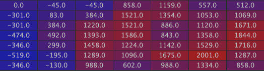
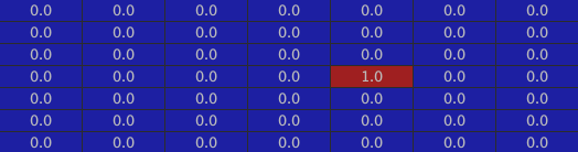
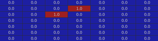
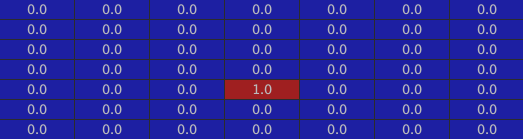
Now let us apply the convolution with the first convolution kernel (use the same kernel for the 3 input channels) to obtain our first new channel:
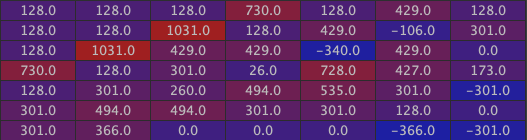
The maximal values are in bright red. Observe as the two maximal numbers are precisely localized on the left part of the roof.
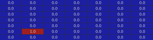
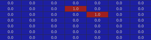
Here is the second new channel (with the second convolution kernel used for the 3 input channels):
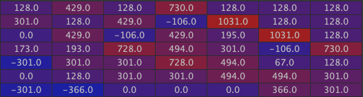
Note as here, the maximal numbers are precisely localized on the right part of the roof.
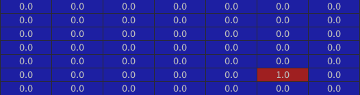
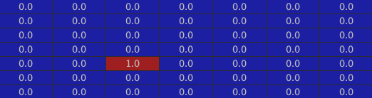
Here is the third one, corresponding to the window:
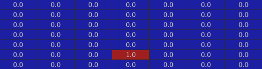
Then the two walls:
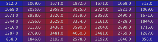
And finally the inside of the house:
L3
In this $ layer $ we will use the trick of the “Biological Neuron” we saw in this article.
First, we add biases to the previous channels. We can make the assumption that this step is in fact included in the convolution (once again, this was already the case for the $ Linear $ case). Concretely, the biases are just numbers that are added to every “pixel” of one chosen channel.
As we have 6 channels coming from the $ L2 $ $ layer $, we must choose 6 biases, each of them being added to every “pixel” of the corresponding channel (the first bias will be added to every “pixel” of the first previous channel, the second bias will be added to every “pixel” of the second previous channel…).
Here are the 6 biases:
\[-1030, -1030, -1990, -2000, -2000, -4059\]Then we use a $ ReLU $ $ activation $ $ layer $. We already saw how it works in the 1D case here: applying the $ activation $ $ function $ to every neuron. In the 2D case, we do the same on every “pixel” of every channels.
This $ L3 $ $ layer $ ($ ReLU $ $ activation $) will produce 6 new channels.
Here are the two corresponding to the house’s roof:
The window:
The walls:
The inside of the house:
L4
$ L4 $ will be a new $ Convolutional $ $ layer $.
We want to build 6 new channels, but there are 6 channels coming from the $ L3 $ $ layer $. This means that we should choose $ 6 * 6 = 36 $ different convolution kernels! We will use another trick to choose the 36 different kernels.
For each group of 6 kernels, we will suppose that only one does not contain only 0 in it. To build the first new channel, we will suppose that the first kernel does not contain only 0 (the other 5 kernels containing only 0). To build the second new channel, we will suppose that the second kernel does not contain only 0 (the other 5 kernels containing only 0). Same logic for the other new channels.
Now for the list of the different convolution kernels that do not contain 0:
\[\begin{bmatrix} 0 & 0 & 0 \\ 1 & 0 & 0 \\ 0 & 0 & 0 \end{bmatrix} \begin{bmatrix} 0 & 0 & 0 \\ 0 & 0 & 1 \\ 0 & 0 & 0 \end{bmatrix}\] \[\begin{bmatrix} 0 & 0 & 0 \\ 0 & 1 & 0 \\ 0 & 0 & 0 \end{bmatrix}\] \[\begin{bmatrix} 0 & 0 & 0 \\ 0 & 0 & 0 \\ 1 & 0 & 0 \end{bmatrix} \begin{bmatrix} 0 & 0 & 0 \\ 0 & 0 & 0 \\ 0 & 0 & 1 \end{bmatrix}\] \[\begin{bmatrix} 0 & 0 & 0 \\ 0 & 0 & 0 \\ 0 & 1 & 0 \end{bmatrix}\]This $ L4 $ $ layer $ will produce 6 new channels.
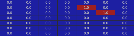
Here are the two corresponding to the house’s roof:
The window:
The walls:
The inside of the house:
L5
$ L5 $ will be a new $ Convolutional $ $ layer $.
We want to build the final most abstract channel. As there are 6 channels coming from the $ L4 $ $ layer $, we must choose $ 1 * 6 = 6 $ different convolution kernels.
Here are they:
\[\begin{bmatrix} 1 & 0 & 0 \\ 0 & 0 & 0 \\ 0 & 0 & 0 \end{bmatrix} \begin{bmatrix} 0 & 0 & 1 \\ 0 & 0 & 0 \\ 0 & 0 & 0 \end{bmatrix}\] \[\begin{bmatrix} 0 & 0 & 0 \\ 0 & 0 & 1 \\ 0 & 0 & 0 \end{bmatrix}\] \[\begin{bmatrix} 0 & 0 & 0 \\ 0 & 0 & 0 \\ 1 & 0 & 0 \end{bmatrix} \begin{bmatrix} 0 & 0 & 0 \\ 0 & 0 & 0 \\ 0 & 0 & 1 \end{bmatrix}\] \[\begin{bmatrix} 0 & 0 & 0 \\ 0 & 0 & 0 \\ 0 & 1 & 0 \end{bmatrix}\]Let us recall the different channels coming from $ L4 $:
- the first two channels represent the “left roof” and the “right roof”
- the third represents the “window”
- the fourth and fifth represent the “left” and “right walls”
- the sixth represents the “inside of the house”
We can now “translate” what the meaning of the final channel will be:
- The first kernel is associated to the first input channel, it triggers on “pixels” where the top left hand corner neighbour is a “left roof”
- The second kernel is associated to the second input channel, it triggers on “pixels” where the top right hand corner neighbour is a “right roof”
- The third kernel triggers on “pixels” where the right neighbour is a “window”
- The fourth kernel triggers on “pixels” where the bottom left hand corner neighbour is a “ left wall”
- The fifth kernel triggers on “pixels” where the bottom right hand corner neighbour is a “right wall”
- The sixth kernel triggers on “pixels” where the bottom neighbour is the “inside of the house”
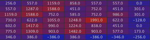
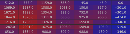
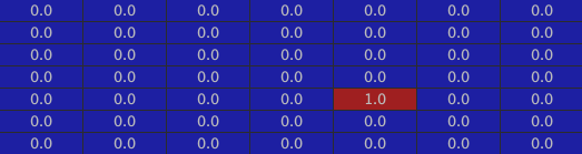
In fact, there is a precise localisation where these 6 statements are all true at once: the exact center. Applying the convolution to the center “pixel”, we find : $ 1 + 1 + 1 + 1 + 1 + 1 = 6 $ coming from the different kernels application on their corresponding channels.
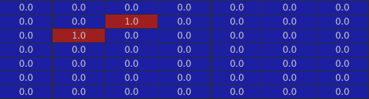
Indeed if we take a look at the final channel, we have:
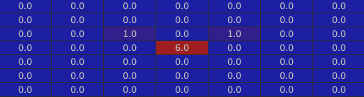
We could add one bias and a final $ ReLU $ $ layer $ to obtain a cleaner channel with just the center “pixel” triggered (same idea as $ L3 $) but we have already understood that it is the maximal activation that particularly interests us.
We have built a $ model $ composed of 5 $ layers $, our biggest so far!
It is time to summarize what a house is for our $ model $. According to the final channel representing the “house”, there are multiple “pixels” that may be a “house” (potentially each “pixel” in the grid). But the center “pixel” is the most triggering “pixel”: every kernel is triggered by their associated channel at this localization. Said differently a “house” “pixel” has:
- a “left roof” (first previous channel) as top left hand corner neighbour (first kernel)
- a “right roof” (second previous channel) as top right hand corner neighbour (second kernel)
- a “window” (third previous channel) as right neighbour (third kernel)
- a “left wall” (fourth previous channel) as bottom left hand corner neighbour (fourth kernel)
- a “right wall” (fifth previous channel) as bottom right hand corner neighbour (fifth kernel)
- the “inside of a house” (sixth previous channel) as bottom neighbour (sixth kernel)
Conclusion
In this article, we saw that an image is a type of data that is not structured in itself. In order to understand such low level information, one has to build “abstract” representations that progressively build sense.
The $ Convolution $ is an operation that combines representations, capturing spatial particularities. It links the semantic together with space.
Nonetheless, the different kernels we used were given “out of nowhere”. In the next article, we will see what is missing in order for these kernels to be learned by the $ model $ itself.