Weights' Balancing
Introduction
In the linear layer and activation layer articles, we saw how to compute the forward pass and the backward pass of the different $ layers $ that compose the $ model $ introduced in the “Example” of the second article.
In this article we will consider this simple $ model $ in order to illustrate the balance that occurs after each weights update of the gradient descent algorithm. This balance enables to compensate the difference between the $ model $’s produced result and the expected one. The final goal being to minimize this difference over the time (read the loss function article).
Example
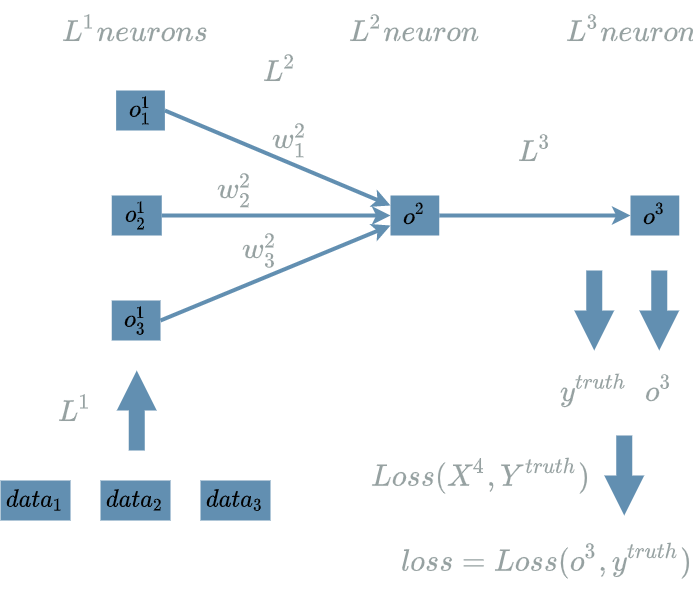
Here is the neural structure synthesis during the forward pass of our simple $ model $:
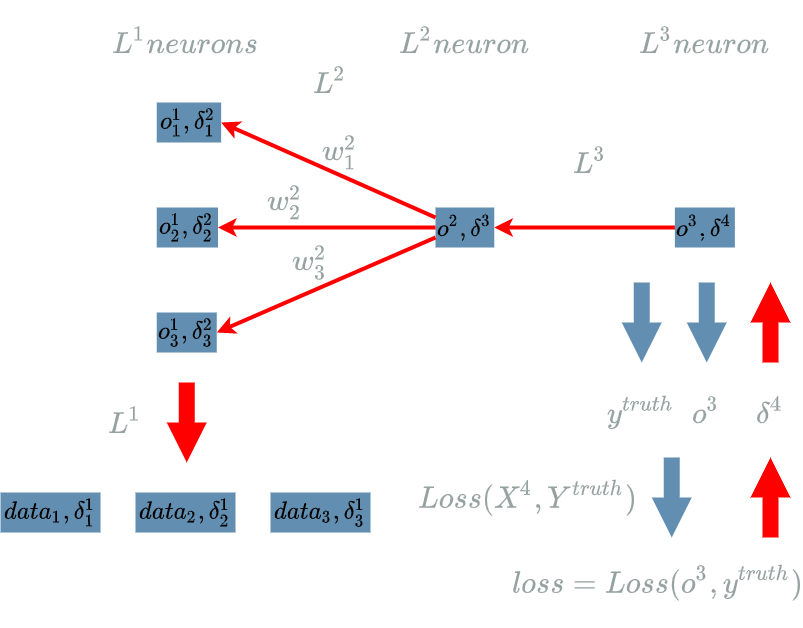
And below is the neural structure during its backward pass:
Sign Flow Analysis
Let us recap the main steps of the training phase we introduced in the first article. These steps have been called the gradient descent algorithm:
- pick one data input in the dataset
- run the forward pass for the $ model $ on this data input
- use the $ Loss $ function to compute the error between the result produced by the $ model $ and the expectation given by the data output
- run the backward pass to compute:
- the learning flow
- the $ derivative $ of the $ Loss $ function according to $ W $
- update the weights of $ model $
We saw in the weights article that the learning flow sole purpose is to be able to compute $ \delta w $ in the weights update formula:
\[\hat{w} = w - \alpha . \delta w\]In the same article, we also saw how this $ -\delta w $ is the direction of update and $ \alpha $ the length of the update.
Still, $ \alpha $ is not that important, we know it must be very little so that the many epochs we run during the gradient descent algorithm will progressively minimize the $ Loss $ function.
The really important part of the update formula is the direction of update: $ -\delta w $, and especially its sign.
This is the reason why we will now analyze the effect of the sign of the final $ loss $ on the sign of $ \delta w $. This analyze will illustrate the impact notion we have been dealing with since the loss function article.
But before that, we have to follow the order of the backward pass because we know the importance of the learning flow in order to compute $ \delta w $.
Let us first analyze the sign back propagation of the learning flow so that we will finally be able to analyze the impact on the weights update:
In our Example, the order of the backward pass is: $ Loss $ -> $ L3 $ -> $ L2 $ -> $ L1 $, so let us begin with the $ Loss $ sign flow.
Loss Sign Flow
Let us recap the formula of the $ Loss $ function we have used in the loss function article:
\[Loss(X^4, Y^{truth}) = \frac{1}{2} (X^4 - Y^{truth})^2\]In the same article we saw how this $ Loss $ serves a “systematic way of telling the $ model $ what is right or wrong”. And from the backward pass article we introduced the learning flow and we computed it for this $ Loss $ function:
\[\delta^4 = o^3 - y^{truth}\]What it is interesting to note is how “pure” this formula is. The learning flow for the $ Loss $ function just compares the actual output of $ model $ with the expected output $ y^{truth} $. But if we look closer at the formula for the $ Loss $ function, we may see how “artificial” it is: it has been chosen so that its $ derivative $ gives a good looking $ \delta^4 $ . [1]
It appears that the whole $ Loss $ function is “just a global indicator”. What really is propagated during the training phase is the learning flow. Thanks to the simple formula for $ \delta^4 $ it is really easy to understand what happens during the training phase. We have 3 cases to consider for our sign analysis:
- when $ model $ produces $ o^3 = y^{truth} $
- when $ model $ produces $ o^3 < y^{truth} $
- when $ model $ produces $ o^3 > y^{truth} $
$ o^3 = y^{truth} $
\[\delta^4 = o^3 - y^{truth}\]The perfect situation: the $ model $ already produces the expected output, nothing to learn!
\[\boxed{\delta^4 = 0}\]$ o^3 < y^{truth} $
\[\delta^4 = o^3 - y^{truth}\]The $ model $ produces a lower than expected output.
\[\boxed{\delta^4 < 0}\]$ o^3 > y^{truth} $
\[\delta^4 = o^3 - y^{truth}\]The $ model $ produces a higher than expected output. It is the same case as in the previous paragraph but with the opposite impact!
\[\boxed{\delta^4 > 0}\]L3 Sign Flow
$ L3 $ is a $ ReLU $ $ activation $ $ layer $ with 1 output neuron. In the previous article, we found:
\[\delta^{3} = \delta^{4} \text{ if } o^2 \geq 0 \text{ else 0 }\]Let us cover the 3 cases coming from the previous paragraph:
- when $ model $ produces $ o^3 = y^{truth} $ => $ \delta^4 = 0 $
- when $ model $ produces $ o^3 < y^{truth} $ => $ \delta^4 < 0 $
- when $ model $ produces $ o^3 > y^{truth} $ => $ \delta^4 > 0 $
$ \delta^4 = 0 $
\[\delta^{3} = \delta^{4} \text{ if } o^2 \geq 0 \text{ else 0 }\]As we saw in this paragraph, we have nothing to learn in this situation. Without any surprise we have:
\[\boxed{\delta^3 = 0}\]$ \delta^4 < 0 $
\[\delta^{3} = \delta^{4} \text{ if } o^2 \geq 0 \text{ else 0 }\]In this situation, we must beware of the sign of $ o^2 $:
$ o^2 \geq 0$
\[\boxed{\delta^3 < 0}\]$ o^2 < 0$
\[\boxed{\delta^3 = 0}\]We are in a bad situation when $ o^2 < 0 $, we are blocking the learning flow while there is something to learn: $ \delta^4 < 0 $. We should definitely avoid this situation and think where the problem comes from in the first place.
Let us look back at the $ L3 $ formula:
\[L3(X^3) = X^3 \text{ if } X^3 \geq 0 \text{ else } 0\]Immediately we find the culprit: “$ \text{ if } X^3 \geq 0 \text{ else } 0 $”. We should think why we introduced it in the activation article. There were 3 reasons to use an $ activation $ function:
- transform value ranges
- add a non linearity in the $ model $ to increase its expressiveness
- mimic the activation potential in biology
The $ ReLU $ activation main interests are the 2 and 3. But it is really the 3 that causes our bad situation. This point has not been discussed very much yet, we will adress it in the next article. Still, we could preserve the 2 using another $ activation $ function like the $ leaky $ $ ReLU $:
\[leaky \text{ } ReLU(x) = \left\{\begin{align} x, & \text{ if $x \geq 0$}\\ 0.01x, & \text{ otherwise} \end{align} \right.\]With such an $ activation $ function, we would have computed:
\[\delta^{3} = \left\{\begin{align} \delta^4, & \text{ if $o^2 \geq 0$}\\ 0.01. \delta^4, & \text{ otherwise} \end{align} \right.\]Our result would have been:
\[\delta^{3} < 0\]and not
\[\delta^{3} = 0\]while preserving the non linearity.
In order to avoid this bad situation we will assume that $ \delta^4 < 0 => \delta^3 < 0 $.
$ \delta^4 > 0 $
\[\delta^{3} = \delta^{4} \text{ if } o^2 \geq 0 \text{ else 0 }\]$ o^2 \geq 0$
\[\boxed{\delta^3 > 0}\]$ o^2 < 0$
\[\boxed{\delta^3 = 0}\]When $ o^2 < 0 $, we have the same bad situation as in this paragraph.
In order to avoid this bad situation we will assume that $ \delta^4 > 0 => \delta^3 > 0 $.
L2 Sign Flow
$ L2 $ is a $ Linear $ $ layer $ with 1 output neuron. In the linear layer article, we found:
\[\delta^{2} = \delta^{3} . w^2\]Let us cover the 3 cases coming from the previous paragraph:
- when $ model $ produces $ o^3 = y^{truth} $ => $ \delta^3 = 0 $
- when $ model $ produces $ o^3 < y^{truth} $ => $ \delta^3 < 0 $
- when $ model $ produces $ o^3 > y^{truth} $ => $ \delta^3 > 0 $
$ \delta^3 = 0 $
\[\delta^{2} = \delta^{3} . w^2\]As we saw in this paragraph, we have nothing to learn in this situation.
\[\boxed{\delta^{2} = 0}\]$ \delta^3 < 0 $
In this situation, we must beware of the sign of $ w^2 $.
\[sign(\delta^{2}) = sign(\delta^{3}) . sign(w^2)\] \[\boxed{sign(\delta^{2}) = -sign(w^2)}\]$ \delta^3 > 0 $
In this situation, we must beware of the sign of $ w^2 $.
\[sign(\delta^{2}) = sign(\delta^{3}) . sign(w^2)\] \[\boxed{sign(\delta^{2}) = sign(w^2)}\]L1 Sign Flow
$ L1 $ is an $ Input \text{ } 1D $ $ layer $ with 3 output neurons. In the activation layer article, we found:
\[\delta^{1} = \delta^{2}\]$ \delta^2 = 0 $
\[\boxed{\delta^{1} = 0}\]$ \delta^2 < 0 $
\[\boxed{\delta^{1} < 0}\]$ \delta^2 > 0 $
\[\boxed{\delta^{1} > 0}\]Update Analysis
We have been able to back propagate the sign of the learning flow when having lower results than expected or higher results than expected in the order of the backward pass.
We are now ready to analyze the impact of these lower/higher results on the weights update.
In our current $ model $ we only have weights in the $ L2 $ $ layer $. Thus we have to update them with the formula we already saw:
\[\hat{w^2} = w^2 - \alpha . \delta w^2\]L2 Update
$ L2 $ is a $ Linear $ $ layer $ with 1 output neuron. In the linear layer article, we found:
\[\delta w^{2} = \delta^{3} . o^1\]We are now able to replace $ \delta w^2 $ in the below formula:
\[\hat{w^2} = w^2 - \alpha . \delta w^2\]Let us cover the 3 cases coming from the sign flow analysis:
- when $ model $ produces $ o^3 = y^{truth} $ => $ \delta^3 = 0 $
- when $ model $ produces $ o^3 < y^{truth} $ => $ \delta^3 < 0 $
- when $ model $ produces $ o^3 > y^{truth} $ => $ \delta^3 > 0 $
$ \delta^3 = 0 $
As we saw in this paragraph, we have nothing to learn in this situation.
\[\begin{align} \delta w^{2} &= \delta^{3} . o^1 \\ &= 0 \end{align}\]Thanks to the update formula, we know the weights will be:
\[\hat{w^2} = w^2 - \alpha . \delta w^2\] \[\boxed{\hat{w^2} = w^2}\]This is on par with the fact that there is nothing to learn in this situation.
$ \delta^3 < 0 $
In this situation, we must beware of the sign of $ o^1 $.
$ o^1 \geq 0 $
\[\begin{align} \hat{w^2} &= w^2 - \alpha . \delta w^2 \\ &= w^2 - \alpha . \delta^{3} . o^1 \end{align}\] \[\boxed{\hat{w^2} \geq w^2}\]$ o^1 < 0 $
\[\begin{align} \hat{w^2} &= w^2 - \alpha . \delta w^2 \\ &= w^2 - \alpha . \delta^{3} . o^1 \end{align}\] \[\boxed{\hat{w^2} < w^2}\]$ \delta^3 > 0 $
In this situation, we must beware of the sign of $ o^1 $.
$ o^1 \geq 0 $
\[\begin{align} \hat{w^2} &= w^2 - \alpha . \delta w^2 \\ &= w^2 - \alpha . \delta^{3} . o^1 \end{align}\] \[\boxed{\hat{w^2} \leq w^2}\]$ o^1 < 0 $
\[\begin{align} \hat{w^2} &= w^2 - \alpha . \delta w^2 \\ &= w^2 - \alpha . \delta^{3} . o^1 \end{align}\] \[\boxed{\hat{w^2} > w^2}\]Balancing the Weights
In this paragraph we illustrate the balance behind the weights updates computed in the previous paragraph.
First of all let us recap the different situations we have for our $ \hat{w^2} $ update:
| situation | model result | $ \hat{w^2} $ |
|---|---|---|
| $ \delta^3 = 0 $ | as expected | keep same $ w^2 $ |
| $ \delta^3 < 0 $ and $ o^1 \geq 0 $ | lower than expected | increase $ w^2 $ |
| $ \delta^3 < 0 $ and $ o^1 < 0 $ | lower than expected | decrease $ w^2 $ |
| $ \delta^3 > 0 $ and $ o^1 \geq 0 $ | higher than expected | decrease $ w^2 $ |
| $ \delta^3 > 0 $ and $ o^1 < 0 $ | higher than expected | increase $ w^2 $ |
Let us go back to the $ L2 $ $ layer $ definition:
\[\begin{align} L2(X^2, W^2) &= W^2 . X^2 & \text{ with } X^2 = (X^2_1, X^2_2, X^2_3) \\ & & \text{ and } W^2 = (W^2_1, W^2_2, W^2_3) \\ &= W^2_1 . X^2_1 + W^2_2 . X^2_2 + W^2_3 . X^2_3 \\ \end{align}\]Said differently:
\[o^2 = w^2_1 . o^1_1 + w^2_2 . o^1_2 + w^2_3 . o^1_3\]In the array above, we spoke about $ w^2 $ but in fact there are several weights: $ w^2_1 $, $ w^2_2 $, $ w^2_3 $. In order to fix the ideas, we will concentrate on one of them: $ w^2_1 $. The exact same logic applies for the others.
$ \delta^3 = 0 $
This is the ideal situation, it is no wonder we must keep the same value for $ w^2_1 $.
$ \delta^3 < 0 $ and $ o^1 \geq 0 $
The $ model $ produces a lower than expected output. The update formula tells us we must increase $ w^2_1 $.
The crucial part to understand why is to go back to the meaning of $ \delta^3 < 0 $. First of all, let us recall the backward pass article:
\[\delta^3 = \frac{\partial Loss}{\partial X^3}(o^2)\]Now, thanks to “The Derivative of the Loss Function” of the loss function article we can paraphrase $ \delta^3 $ as: “the impact of $ X^3 $ on the $ Loss $ function when evaluated on $ o^2 $”.
We conclude that the fact that $ \delta^3 < 0 $ implies that a small increase in $ o^2 $ would decrease the value of $ loss $, which is actually our goal !
We are now able to better understand our current situation:
- As $ \delta^3 < 0 $, we would like $ o^2 $ to increase in order for $ loss $ to decrease
- But $ o^2 $ depends on $ o^1_1 \geq 0 $
- And in order to know the best new value for $ w^2_1 $ we consider every other terms to be fixed
That way, it is clear that $ w^2_1 $ must be increased so that $ o^2 = w^2_1 . o^1_1 + w^2_2 . o^1_2 + w^2_3 . o^1_3 $ increases which is exactly what was computed in the previous paragraph !
$ \delta^3 < 0 $ and $ o^1 < 0 $
Let us go faster now !
The $ model $ now produces a lower than expected output. The update formula tells us we must decrease $ w^2_1 $.
This is logical considering that:
- $ \delta^3 < 0 $ => $ o^2 $ must be increased
- $ o^1_1 < 0 $
- the only part that we can modify is $ w^2_1 $
=> $ w^2_1 $ must be decreased so that $ o^2 = w^2_1 . o^1_1 + w^2_2 . o^1_2 + w^2_3 . o^1_3 $ increases.
$ \delta^3 > 0 $ and $ o^1 \geq 0 $
The $ model $ produces a higher than expected output. The update formula tells us we must decrease $ w^2_1 $.
This is logical considering that:
- $ \delta^3 > 0 $ => $ o^2 $ must be decreased
- $ o^1_1 \geq 0 $
- the only part that we can modify is $ w^2_1 $
=> $ w^2_1 $ must be decreased so that $ o^2 = w^2_1 . o^1_1 + w^2_2 . o^1_2 + w^2_3 . o^1_3 $ decreases.
$ \delta^3 > 0 $ and $ o^1 < 0 $
The $ model $ produces a higher than expected output. The update formula tells us we must increase $ w^2_1 $.
This is logical considering that:
- $ \delta^3 > 0 $ => $ o^2 $ must be decreased
- $ o^1_1 < 0 $
- the only part that we can modify is $ w^2_1 $
=> $ w^2_1 $ must be increased so that $ o^2 = w^2_1 . o^1_1 + w^2_2 . o^1_2 + w^2_3 . o^1_3 $ decreases.
Back to the Learning Flow
There are 2 paragraphs that were not used during our update analysis: the L2 Sign Flow and the L1 Sign Flow paragraphs.
In fact we have already seen this aspect but the learning flow’s only purpose is to be able to compute $ \delta w $. In our current example, the $ L2 $ $ layer $ is the only one to have weights. Hence, the learning flow back propagation is necessary until we get $ \delta^3 $.
If we look back at the last diagram of the first paragraph,
it is clear we just have to compute the learning flow
for $ Loss $ and for the $ L3 $ $ layer $.
This means we could have skipped the computation of the learning flow for $ L2 $ and for $ L1 $ in the
backward pass article ![]()
Conclusion
In the balancing the weights paragraph, we illustrated that the weights update comes from the fact that the final result is too high or too low compared to the expected result and that the weights are the only “moving part” (see the weights article) to compensate. From there, the learning flow just helps cascading the impact on the different intermediate levels.
In the next article we will consider the global function of our simple $ model $ operating on the data input.
In fact there is another reason to use this formula for the $ Loss $ function:
\[Loss(X^4, Y^{truth}) = \frac{1}{2} (X^4 - Y^{truth})^2\]The “square” in the formula adds an interesting property: the $ Loss $ function is convex. This guaranties that the minimum we are finding with our gradient descent algorithm will be the global minimum of the whole function. ↑