The Backward Pass

Introduction

In the previous article, we began to compute the different $ derivative $ functions of $ Loss $ but we were stuck early in the process: we could only compute $ \delta 4 = \frac{\partial Loss}{\partial X^4}(o3, y^{truth}) $. Indeed, we had the explicit formula linking $ X^4 $ to $ Loss $ and we were able to compute an explicit formula for $ \frac{\partial Loss}{\partial X^4} $.

But our $ model $ is composed of other variables and we must compute the impact of each and every of them on $ Loss $. The reason for that will be explained in the next article.

In this article we will see how the structure in $ layers $ of our $ model $ helps us computing the impacts of the inner variables of the $ model $ on the $ Loss $ function.

The Backward Pass

Before diving into some more computation, let us talk about the forward pass once more (first referenced here). It has a nemesis in the backward pass that plays the exact opposite role.

The forward pass propagates the information flow through the different layers from the input layer to the output layer. The backward pass is about a reversed signal that we could call the learning flow. This signal is back propagated from the output layer to the input layer.

From now on, we will keep in mind that the learning flow is in fact the $ derivative $ of $ Loss $ according to the $ X $ variable:

\[\boxed{\frac{\partial Loss}{\partial X}}\]

We note $ \delta $ when we evaluate this function on $ x $ data from a dataset and $ y^{truth} $ the associated expectation:

\[\boxed{\delta = \frac{\partial Loss}{\partial X}(x, y^{truth})}\]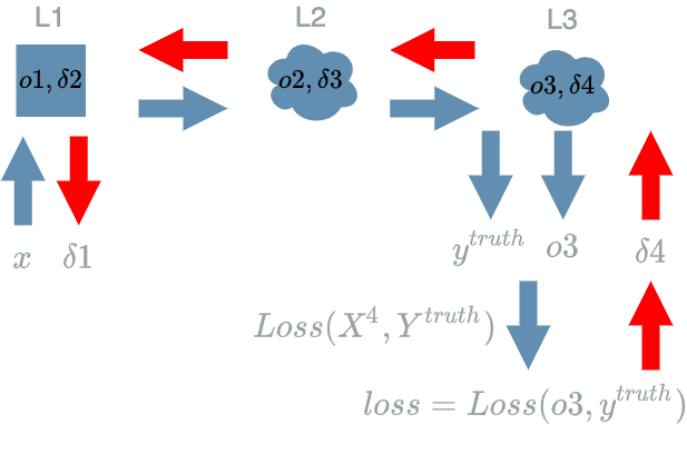

If the input layer is the place where the data input is initialised by the developer in the forward pass, it is clear from the early computations we made ($ \delta 4 $) in the previous article that the $ Loss $ function is the place where the backward pass is initialised.

There is a final difference between the two: the forward pass is run during the training phase and the inferring phase (see “Training, Inferring” in the first article) while the backward pass is only run during the training phase, which comforts its signal naming of learning flow.

A Closer Look at one Layer

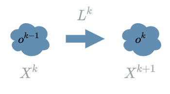
To be a little more specific, we can take a look at some $ L^{k} $ $ layer $ in particular. By definition we have an explicit formula for $ L^{k}(X^{k}) $ function. Running its forward pass is easy: we just consider that the previous result $ o^{k-1} $ has already been computed. This enables us to compute $ o^{k} = L^{k}(o^{k-1}) $.

But for the backward pass we do the reverse logic. We must consider we already have computed the “future” learning flow $ \delta^{k+1} $ and we want to propagate the learning flow through $ L^{k} $, computing $ \delta^{k} $.

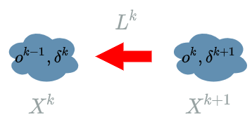
In order to compute $ \delta^{k} $ we proceed in two steps:

1. We compute an explicit formula for $ \frac{\partial Loss}{\partial X^{k}} $.
2. We evaluate this function on $ o^{k-1} $.

The most difficult point is the 1 because we must compute the link between $ X^{k} $ and $ Loss $ which is “chained”. There are 2 essential parts in that “chain”:

• The link between $ X^k $ and $ X^{k+1} $, given by the definition o:f $ L^{k} $: $ X^{k+1} = L^{k}(X^{k}) $.
• The link between $ X^{k+1} $ and $ Loss $ which is the “future” learning flow: $ \delta^{k+1} $.

When we have these two parts, we may use the chain rule…

The Chain Rule

In the previous paragraph, we have seen the two essential parts to obtain the explicit formula for:

\[\frac{\partial Loss}{\partial X^k}\]

In this paragraph we will see how to compose them in order to establish the link between $ X^k $ and $ Loss $ when $ X^k $ is an inner variable (when $ X^k $ is a final variable we already saw how to proceed in the previous article).

In fact we have to use the chain rule, here on Wikipedia:

“If a variable z depends on the variable y, which itself depends on the variable x (that is, y and z are dependent variables), then z depends on x as well, via the intermediate variable y. In this case, the chain rule is expressed as

\[\frac{dz}{dx} = \frac{dz}{dy}.\frac{dy}{dx}\]

and

\[\frac{dz}{dx} \bigg\rvert_{x} = \frac{dz}{dy} \bigg\rvert_{y(x)} . \frac{dy}{dx} \bigg\rvert_{x}\]

for indicating at which points the derivatives have to be evaluated.”

Using the chain rule with $ z = Loss $ and $ y = L^{k} $, the formula becomes:

\[\frac{\partial Loss}{\partial X^{k}} = \frac{\partial Loss}{\partial L^{k}} . \frac{\partial L^{k}}{\partial X^{k}}\]

Thanks to the forward pass we know that $ X^{k+1} = L^{k}(X^{k}) $, so we get:

\[\boxed{\frac{\partial Loss}{\partial X^{k}} = \frac{\partial Loss}{X^{k+1}} . \frac{\partial L^{k}}{\partial X^{k}}}\]

where $ \frac{\partial Loss}{X^{k+1}} $ is the “future” learning flow we have already computed and $ \frac{\partial L^{k}}{\partial X^{k}} $ is a part we compute thanks to some formula we learnt at school.

mathematically shy people should jump to the conlusion

Example

We are now able to end the computations we began in the last paragraph of the previous article !

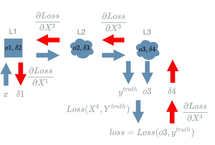
Computing $ \frac{\partial Loss}{\partial X^3} $

We are looking for a link between $ X^3 $ and $ Loss $. As the backward pass suggests, we have to use what we have already computed: $ \delta 4 = \frac{\partial Loss}{\partial X^4}(o3, y^{truth}) $ and what directly uses $ X^3 $ which is $ L3 $: $ L3(X^3) = X^3 \text{ if } X^3 \geq 0 \text{ else } 0 $.

Then we are able to use the chain rule with $ z = Loss $ and $ y = L3 $, the formula becomes:

\[\boxed{\frac{\partial Loss}{\partial X^3} = \frac{\partial Loss}{\partial L3} . \frac{\partial L3}{\partial X^3}}\]

Thanks to the forward pass we know that $ X^4 = L3(X^3) $, so we have:

\[\frac{\partial Loss}{\partial L3} = \frac{\partial Loss}{\partial X^4} \text{ we recognize a learning flow !}\]

and:

\[\begin{align} \frac{\partial L3}{\partial X^3} &= \frac{\partial (X^3 \text{ if } X^3 \geq 0 \text{ else } 0)}{\partial X^3} \text{ with the definition of } L3(X^3) \\ &= 1 \text{ if } X^3 \geq 0 \text{ else } 0 \end{align}\]

Assembling those results:

\[\begin{align} \frac{\partial Loss}{\partial X^3} &= \frac{\partial Loss}{\partial L3} . \frac{\partial L3}{\partial X^3} \\ &= (\frac{\partial Loss}{\partial X^4}) * (1 \text{ if } X^3 \geq 0 \text{ else } 0) \\ &= \frac{\partial Loss}{\partial X^4} \text{ if } X^3 \geq 0 \text{ else } 0 \end{align}\]

We can now evaluate this function on the values that have produced the final $ loss $, let $ \delta 3 $ be this result:

\[\begin{align} \delta 3 &= \frac{\partial Loss}{\partial X^3}(o2) \\ &= \frac{\partial Loss}{\partial X^4}(o3, y^{truth}) \text{ if } o2 \geq 0 \text{ else } 0 \\ &= \delta 4 \text{ if } o2 \geq 0 \text{ else } 0 \end{align}\]

We have found:

\[\boxed{\delta 3 = \frac{\partial Loss}{\partial X^3}(o2) = \delta 4 \text{ if } o2 \geq 0 \text{ else } 0}\]

Computing $ \frac{\partial Loss}{\partial X^2} $

We are looking for a link between $ X^2 $ and $ Loss $. As the backward pass suggests, we have to use what we have already computed: $ \delta 3 = \frac{\partial Loss}{\partial X^3}(o2) $ and what directly uses $ X^2 $ which is $ L2 $: $ L2(X^2) = \frac{1}{200} X^2_1 - \frac{3 000}{11 600 000} X^2_2 + \frac{1}{5 800} X^2_3 \text{, with } X^2 = (X^2_1, X^2_2, X^2_3) $.

We have one problem though, it is that: $ X^2 = (X^2_1, X^2_2, X^2_3) $. And we told in the introduction that we want to compute the impact of each and every variable of $ model $ on the $ Loss $ function. This means we have to compute the $ derivative $ functions of $ Loss $ according to each of them:

\[\frac{\partial Loss}{\partial X^2_1} \text{, } \frac{\partial Loss}{\partial X^2_2} \text{, and } \frac{\partial Loss}{\partial X^2_3}\]

We are able to use the chain rule with $ z = Loss $ and $ y = L2 $, for $ X^2_1 $ the formula becomes:

\[\boxed{\frac{\partial Loss}{\partial X^2_1} = \frac{\partial Loss}{\partial L2} . \frac{\partial L2}{\partial X^2_1}}\]

Thanks to the forward pass we know that $ X^3 = L2(X^2) $, so we have:

\[\frac{\partial Loss}{\partial L2} = \frac{\partial Loss}{\partial X^3} \text{ we recognize a learning flow !}\]

and:

\[\begin{align} \frac{\partial L2}{\partial X^2_1} &= \frac{\partial (\frac{1}{200} X^2_1 - \frac{3 000}{11 600 000} X^2_2 + \frac{1}{5 800} X^2_3)}{\partial X^2_1} \text{ with the definition of } L2(X^2) \\ &= \frac{1}{200} \end{align}\]

Assembling those results:

\[\begin{align} \frac{\partial Loss}{\partial X^2_1} &= \frac{\partial Loss}{\partial L2} . \frac{\partial L2}{\partial X^2_1} \\ &= (\frac{\partial Loss}{\partial X^3}) * (\frac{1}{200}) \end{align}\]

We can now evaluate this function on the values that have produced the final $ loss $, let $ \delta 2_1 $ be this result:

\[\begin{align} \delta 2_1 &= \frac{\partial Loss}{\partial X^2_1}(o1) \\ &= \frac{\partial Loss}{\partial X^3}(o2) * \frac{1}{200} \\ &= \delta 3 * \frac{1}{200} \end{align}\]

We have found:

\[\delta 2_1 = \frac{\partial Loss}{\partial X^2_1}(o1) = \delta 3 * \frac{1}{200}\]

We do the same to compute:

\[\delta 2_2 = \frac{\partial Loss}{\partial X^2_2}(o1) = \delta 3 * (-\frac{3 000}{11 600 000})\]

and

\[\delta 2_3 = \frac{\partial Loss}{\partial X^2_3}(o1) = \delta 3 * \frac{1}{5 800}\]

These 3 formulas can be summarized because:

\[\begin{align} \delta 2 &= \frac{\partial Loss}{\partial X^2}(o1) \\ &= (\frac{\partial Loss}{\partial X^2_1}(o1), \frac{\partial Loss}{\partial X^2_2}(o1), \frac{\partial Loss}{\partial X^2_3}(o1)) \\ &= (\delta 2_1, \delta 2_2, \delta 2_3) \\ &= (\delta 3 * \frac{1}{200}, \delta 3 * (-\frac{3 000}{11 600 000}), \delta 3 * \frac{1}{5 800}) \\ &= \delta 3 * (\frac{1}{200}, -\frac{3 000}{11 600 000}, \frac{1}{5 800}) \end{align}\]

We finally have:

\[\boxed{\delta 2 = \frac{\partial Loss}{\partial X^2}(o1) = \delta 3 * (\frac{1}{200}, -\frac{3 000}{11 600 000}, \frac{1}{5 800})}\]

Computing $ \frac{\partial Loss}{\partial X^1} $

We are looking for a link between $ X^1 $ and $ Loss $. As the backward pass suggests, we have to use what we have already computed: $ \delta 2 = \frac{\partial Loss}{\partial X^2}(o1) $ and what directly uses $ X^1 $ which is $ L1 $: $ L1(X^1) = X^1 \text{, with } X^1 = (X^1_1, X^1_2, X^1_3) $.

We have the same problem as in the previous paragraph: $ X^1 = (X^1_1, X^1_2, X^1_3) $. We told in the introduction that we want to compute the impact of each and every variable of $ model $ on the $ Loss $ function. This means we have to compute the $ derivative $ functions of $ Loss $ according to each of them:

\[\frac{\partial Loss}{\partial X^1_1} \text{, } \frac{\partial Loss}{\partial X^1_2} \text{, and } \frac{\partial Loss}{\partial X^1_3} \\\]

But now, we have a new problem: we cannot apply the chain rule as before. Indeed, we are in a case where $ L1 $ depends on multiple variables ($ X^1_1 $, $ X^1_2 $, $ X^1_3 $) and produces multiple variables ($ L1(X^1_1) $, $ L1(X^1_2) $, $ L1(X^1_3) $). So what is the problem ?

Let us concentrate on the impact of $ X^1_1 $ on the $ Loss $ function. Because $ L1 $ is producing 3 variables, this $ X^1_1 $ could impact each of these 3 output variables !

Thus we cannot use the chain rule . ^[1] Are we going to use another formula ? No because we can think in terms of impacts. If we go back to our problem, we have $ X^1_1 $ that could impact three output variables: $ L1(X^1_1) $, $ L1(X^1_2) $, $ L1(X^1_3) $.

If we had used the chain rule with $ z = Loss $ and $ y = L1 $, for $ X^1_1 $ the formula would have been:

\[\frac{\partial Loss}{\partial X^1_1} = \frac{\partial Loss}{\partial L1} . \frac{\partial L1}{\partial X^1_1}\]

But because of the potential impacts of $ X^1_1 $ we have to compute:

\[\boxed{\frac{\partial Loss}{\partial X^1_1} = \frac{\partial Loss}{\partial L1(X^1_1)} . \frac{\partial L1(X^1_1)}{\partial X^1_1} + \frac{\partial Loss}{\partial L1(X^1_2)} . \frac{\partial L1(X^1_2)}{\partial X^1_1} + \frac{\partial Loss}{\partial L1(X^1_3)} . \frac{\partial L1(X^1_3)}{\partial X^1_1}}\]

By chance, it appears that this formula simplifies. Let us recall that $ L1(X^1) = X^1 \text{, with } X^1 = (X^1_1, X^1_2, X^1_3) $. Said differently we have: $ L1((X^1_1, X^1_2, X^1_3)) = (X^1_1, X^1_2, X^1_3) $. Thus we can compute:

\[\begin{align} \frac{\partial L1(X^1_2)}{\partial X^1_1} &= \frac{\partial L1((0, X^1_2, 0))}{\partial X^1_1} \\ &= \frac{\partial ((0, X^1_2, 0))}{\partial X^1_1} \\ &= (0, 0, 0) \end{align}\]

and:

\[\begin{align} \frac{\partial L1(X^1_3)}{\partial X^1_1} &= \frac{\partial L1((0, 0, X^1_3))}{\partial X^1_1} \\ &= \frac{\partial ((0, 0, X^1_3))}{\partial X^1_1} \\ &= (0, 0, 0) \end{align}\]

The simplification of the big formula is:

\[\boxed{\frac{\partial Loss}{\partial X^1_1} = \frac{\partial Loss}{\partial L1(X^1_1)} . \frac{\partial L1(X^1_1)}{\partial X^1_1}}\]

Thanks to the forward pass and the definition of $ L1 $, we know that $ X^2_1 = L1(X^1_1) $, so we have:

\[\frac{\partial Loss}{\partial L1(X^1_1)} = \frac{\partial Loss}{\partial X^2_1} \text{ we recognize a learning flow !}\]

and:

\[\begin{align} \frac{\partial L1(X^1_1)}{\partial X^1_1} &= \frac{\partial ((X^1_1, 0, 0))}{\partial X^1_1} \text{ with the definition of } L1(X^1) \\ &= (1, 0, 0) \end{align}\]

Assembling those results:

\[\begin{align} \frac{\partial Loss}{\partial X^1_1} &= \frac{\partial Loss}{\partial L1(X^1_1)} . \frac{\partial L1(X^1_1)}{\partial X^1_1} \\ &= (\frac{\partial Loss}{\partial X^2_1}) * (1, 0, 0) \end{align}\]

We can now evaluate this function on the values that have produced the final $ loss $, let $ \delta 1_1 $ be this result:

\[\begin{align} \delta 1_1 &= \frac{\partial Loss}{\partial X^1_1}(x) \\ &= \frac{\partial Loss}{\partial X^2_1}(o1) * (1, 0, 0) \\ &= \delta 2_1 * (1, 0, 0) \end{align}\]

We have found:

\[\delta 1_1 = \frac{\partial Loss}{\partial X^1_1}(x) = \delta 2_1 * (1, 0, 0)\]

We do the same to compute:

\[\delta 1_2 = \frac{\partial Loss}{\partial X^1_2}(x) = \delta 2_2 * (0, 1, 0)\]

and

\[\delta 1_3 = \frac{\partial Loss}{\partial X^1_3}(x) = \delta 2_3 * (0, 0, 1)\]

These 3 formulas can be summarized as:

\[\delta 1 = (\delta 2_1, \delta 2_2, \delta 2_3)\]

And finally

\[\boxed{\delta 1 = \delta 2}\]

Conclusion

In this article, we introduced the learning flow which propagates during the backward pass. The order of propagation is the exact reverse as the information flow of the forward pass.

We also had to compute the learning flow because it’s formula is not given by the $ model $ definition as the information flow is.

We may have found those computations scary. And there are two main remedies about that. Either we use an existing framework that will automatically compute the backward pass for us or we choose to fully understand this back propagation.

In the first situation we might lose what is really at the core of learning. Which is the reason why we will spend some time to see a new perspective that should help better understand this backward pass (see the linear layer article).

For now we only keep in mind the general form of the learning flow: it depends on the $ derivative $ of the “current” $ layer $ evaluated on the “previous” outputs multiplied by the “future” $ layer $’s own learning flow (if “current” is $ L^{k} $, “future” would be $ L^{k+1} $ and “previous” would be $ L^{k-1} $).

Finally we did not explain why we computed this learning flow yet ! This is what we will see in the next article

[1]:

In fact the chain rule formula is meant for functions of 1 variable. This is the reason why we see a $ \frac{dz}{dx} $ where we used a partial derivative $ \frac{\partial z}{\partial x} $ in the previous paragraphs. It used to work until now because the $ layers $ considered produced only 1 variable. Hence, the variable we were considering the impact on $ Loss $ was targeting this unique output variable. ↑