Batch Learning
Introduction
In the previous article, we run one epoch of the gradient descent algorithm.
In this article we will explore one new idea to stabilize this algorithm: batch learning.
What is a Batch ?
A batch corresponds to multiple elements of data input taken at once. The main goal is to modify the way our weights are updated so that each update is more robust.
In this article, we talked about the direction to follow in order to update the weights.
With batch learning, we want to update our weights according to the average direction on the batch of data input, let $ \delta w^{avg} $ be it. We can still use the same formula to update the weights as before with this simple replacement:
\[\boxed{\hat{w} = w - \alpha * \delta w^{avg}}\]We are able to modify our gradient descent algorithm so that it is applied on a batch of data input:
- pick a batch of data input in the dataset (just means pick several data input)
- run the forward pass for the $ model $ on each element of the batch
- use the $ Loss $ function to compute the error between the result produced by the $ model $ and the expectation given by the data output, this for each (data input, data output) of the different elements of the batch
- run the backward pass to compute:
- the learning flow for each elements of the batch
- the $ derivative $ of the $ Loss $ function according to $ W $ for each elements of the batch
- update the weights of $ model $ with the average direction $ -\delta w^{avg} $
Do it for all data input in the dataset, we call it an epoch. Repeat for several epochs.
The New Forward Pass
There is no new forward pass, we just have to continue running the forward pass as before, just keeping in mind that the different elements in the batch will be grouped together for learning.
For $ i $ in $ 1, 2 … n $, indices of the batch elements, we compute $ \boxed{model(x^i)} $.
The New Loss Function
From its introduction in the article Loss function, the $ Loss $ function has been used to systematically compare the results produced by the $ model $ with expectations.
Now, we want to compare the results and the expectations on multiple elements of a batch. Each element of the batch being (data input, data output).
One simple idea is to compute the average $ loss $ on these elements.
Example with the $ Loss $ function used in the previous articles where we had picked an $ x $ from the data input and $ y^{truth} $ from the data output and computed:
\[loss = Loss(model(x), y^{truth})\]Now we consider a batch so we have several elements (let us say $ n $ elements):
- $ x^1 $, $ x^2 $, … $ x^n $
- $ y^{truth, 1} $, $ y^{truth, 2} $, … $ y^{truth, n} $
We compute:
\[\begin{align} loss^1 &= Loss(model(x^1), y^{truth, 1}) \\ loss^2 &= Loss(model(x^2), y^{truth, 2}) \\ & \text{...} \\ loss^n &= Loss(model(x^n), y^{truth, n}) \end{align}\]We introduce the average $ Loss^{avg} $ as the average of the errors on the batch:
\[\boxed{Loss^{avg} = \frac{1}{n} . (Loss(model(X^1), Y^{truth, 1}) + Loss(model(X^2), Y^{truth, 2}) + \text{...} + Loss(model(X^n), Y^{truth, n}))}\]and we evaluate this function on real values:
\[loss^{avg} = \frac{1}{n} . (loss^1 + loss^2 + \text{...} + loss^n)\]What is interesting to note is that for any $ X^i $ we have:
\[\frac{\partial Loss^{avg}}{\partial X^i} = \frac{1}{n} . \frac{\partial Loss}{\partial X^i}\]And we recall that $ \frac{\partial Loss}{\partial X^i} $ is used to compute the learning flow.
This means that the new $ Loss^{avg} $ has exactly the same impact on learning as $ Loss^{learning} $, with:
\[\boxed{Loss^{learning}(X, Y^{truth}) = \frac{1}{n} . Loss(X, Y^{truth})}\]In fact $ Loss^{avg} $ is just a global indicator that shows the average error at the end of the forward pass. But what is really propagated during the training phase will be $ Loss^{learning} $.
The New Backward Pass
There is no new backward pass, we just have to continue running the backward pass as before, just keeping in mind that the different elements in the batch will be grouped together for learning.
For $ i $ in $ 1, 2 … n $, indices of the batch elements, we compute:
\[\frac{\partial Loss^{avg}}{\partial X^i}\]and
\[\frac{\partial Loss^{avg}}{\partial W^i}\]Thanks to the previous paragraph, we know it comes down to compute:
\[\boxed{\frac{\partial Loss^{learning}}{\partial X^i} = \frac{1}{n} . \frac{\partial Loss}{\partial X^i}}\]and
\[\boxed{\frac{\partial Loss^{learning}}{\partial W^i} = \frac{1}{n} . \frac{\partial Loss}{\partial W^i}}\]When we evaluate these two functions we have:
\[\delta^{learning} = \frac{1}{n} . \delta\]and
\[\delta w^{learning} = \frac{1}{n} . \delta w\]The State so far
Let us summarize the status so far. We are trying to learn on a batch of (data input, data output). We have to apply the training phase, which is nearly the same as before.
Let us concentrate on one $ L^k $ $ layer $ that declares $ W^k $ weights. Suppose that our batch has $ n $ elements:
- During the forward pass we compute multiple $ o^k $ results, let us say: $ o^{k, 1} \text{, } o^{k, 2} \text{ … } o^{k, n} $.
- During the backward pass we compute multiple $ \delta k^{learning} $ for the learning flow: $ \delta k^{learning, 1} \text{, } \delta k^{learning, 2} \text{ … } \delta k^{learning, n} $.
- During the backward pass we also compute multiple $ \delta w^{k, learning} $: $ \delta w^{k, learning, 1} \text{, } \delta w^{k, learning, 2} \text{ … } \delta w^{k, learning, n} $.
What is common for all these steps is that they are fully independent inside the batch. This means that $ o^{k, 1} $, $ o^{k, 2} $ … $ o^{k, n} $ are fully independent. $ \delta k^{learning, 1} $, $ \delta k^{learning, 2} $ … $ \delta k^{learning, n} $ are fully independent. $ \delta w^{k, learning, 1} $, $ \delta w^{k, learning, 2} $ … $ \delta w^{k, learning, n} $ are fully independent.
The fact that they are fully independent is really interesting in terms of computing: we can fully parallelize their computation inside the current step (forward or backward).
Let us talk about our final goal which is to update the weights according to the average direction $ -\delta w^{avg} $.
For now, this average is clearly out of reach. Indeed, every batch element in the forward pass is isolated from the others. For the backward pass, it is also the case. There is just one modification in the backward pass: the $ \frac{1}{n} $ coefficient in the $ Loss^{learning} $. But clearly this is not sufficient to say we are about to compute an average direction.
The last part where things can get right is the weights update ![]()
Update the Weights: the New Rule
Let us recall the update formula for the weights:
\[\boxed{\hat{w} = w - \alpha * \delta w^{avg}}\]In order to use the update formula we must compute the explicit formula for $ \frac{\partial Loss^{avg}}{\partial W} $ beforehand.
We need to think about the backward pass once more, to understand how $ W $ impacts the final $ Loss $: $ Loss^{avg} $.
Let us consider the $ L^k $ $ layer $ example we introduced in the precedent paragraph. We try to compute an explicit formula for:
\[\frac{\partial Loss^{avg}}{\partial W^k}\]Until now, the values for $ w^k $ have not been updated, they are still the same… This means that every results obtained through the forward pass were not that independent: $ o^{k, 1} $ was computed with $ w^k $ as a value for the $ W^k $. But $ o^{k, 2} $ was computed with the same $ w^k $ value for $ W^k $ … and $ o^{k, n} $ was computed with the same $ w^k $ value for $ W^k $ as well.
Thus $ w^k $ has impacted all batch outputs depending on $ W^k $: $ o^{k, 1}, o^{k, 2} … o^{k, n} $. Said differently, $ W^k $ impacts $ L^k(X^{k, 1}, W^k) $, $ L^k(X^{k, 2}, W^k) $ … and $ L^k(X^{k, n}, W^k) $.
And by definition: $ L^k(X^{k, 1}, W^k) $ impacts $ Loss^{avg} $, $ L^k(X^{k, 2}, W^k) $ impacts $ Loss^{avg} $ … and $ L^k(X^{k, n}, W^k) $ impacts $ Loss^{avg} $.
This comes down to the realization that the same $ w^k $ value is responsible for the final $ loss^{avg} $ through the different batch outputs computed during the forward pass. So in order to have the impact of $ W^k $ on $ Loss^{avg} $ we must simply add the impacts of the different batch outputs:
\[\frac{\partial Loss^{avg}}{\partial W^k} = \frac{\partial Loss^{avg}}{\partial W^{k, 1}} + \frac{\partial Loss^{avg}}{\partial W^{k, 2}} + \text{...} + \frac{\partial Loss^{avg}}{\partial W^{k, n}}\]And we know from this paragraph that:
\[\frac{\partial Loss^{avg}}{\partial W} = \frac{\partial Loss^{learning}}{\partial W}\]This helps us to obtain:
\[\begin{align} \frac{\partial Loss^{avg}}{\partial W^k} &= \frac{\partial Loss^{avg}}{\partial W^{k, 1}} + \frac{\partial Loss^{avg}}{\partial W^{k, 2}} + \text{...} + \frac{\partial Loss^{avg}}{\partial W^{k, n}} \\ &= \frac{\partial Loss^{learning}}{\partial W^{k, 1}} + \frac{\partial Loss^{learning}}{\partial W^{k, 2}} + \text{...} + \frac{\partial Loss^{learning}}{\partial W^{k, n}} \\ &= \frac{1}{n} . (\frac{\partial Loss}{\partial W^{k, 1}} + \frac{\partial Loss}{\partial W^{k, 2}} + \text{...} + \frac{\partial Loss}{\partial W^{k, n}}) \end{align}\]We finally obtained what we were looking for:
$ \frac{\partial Loss^{avg}}{\partial W^k} $ is the average direction of $ \frac{\partial Loss}{\partial W^{k}} $.
Though, we will keep in mind that:
\[\boxed{\frac{\partial Loss^{avg}}{\partial W^k} = \frac{\partial Loss^{learning}}{\partial W^{k, 1}} + \frac{\partial Loss^{learning}}{\partial W^{k, 2}} + \text{...} + \frac{\partial Loss^{learning}}{\partial W^{k, n}}}\]And we evaluate this function:
\[\boxed{\delta w^{k, avg} = \delta w^{k, learning, 1} + \delta w^{k, learning, 2} + \text{...} + \delta w^{k, learning, n}}\]Example
In this example we will start a new training phase from scratch (compared to the “Example: what we do…” in the previous article) but this time with a batch size of 3. If the choice in this example is simple because we have only 3 data input, it may be more touchy in the general case. Yet, there is no magical formula and it will be up to the developer to decide on this parameter. We use the same very small learning rate as before: $ \alpha = 10^{-7} $.
Data
Same data as in the first article.
| data input | data output (expectation) |
|---|---|
| (100 broccoli, 2000 Tagada strawberries, 100 workout hours) | (bad shape) |
| (200 broccoli, 0 Tagada strawberries, 0 workout hours) | (good shape) |
| (0 broccoli, 2000 Tagada strawberries, 3 000 workout hours) | (good shape) |
Model
Same $ model $ as in the weights article.
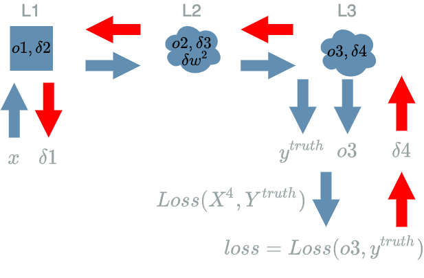
\[\begin{align} L1(X^1) &= X^1 & \text{ with } X^1 = (X^1_1, X^1_2, X^1_3) \\ L2(X^2, W^2) &= W^2 . X^2 & \text{ with } X^2 = (X^2_1, X^2_2, X^2_3) \\ & & \text{ and } W^2 = (W^2_1, W^2_2, W^2_3) \\ &= W^2_1 . X^2_1 + W^2_2 . X^2_2 + W^2_3 . X^2_3 \\ L3(X^3) &= X^3 \text{ if } X^3 \geq 0 \text{ else } 0 \\ \\ model(X) &= L3(L2(L1(X))) & \text{ with } X = (X_1, X_2, X_3) \\ Loss(X^4, Y^{truth}) &= \frac{1}{2} (X^4 - Y^{truth})^2 \end{align}\]We use the initial values for our $ L2 $ weights:
\[w^2 = (\frac{1}{200}, -\frac{3 000}{11 600 000}, \frac{1}{5 800})\]Run the Forward Pass
| $ x $ | $ o1 = L1(x) $ | $ o2 = L2(o1) $ | $ o3 = L3(o2) $ |
|---|---|---|---|
| (100, 2000, 100) | (100, 2000, 100) | (0) | (0) |
| (200, 0, 0) | (200, 0, 0) | (1) | (1) |
| (0, 2000, 3 000) | (0, 2000, 3 000) | (0) | (0) |
| $ o3 = model(x) $ | $ y^{truth} $ = expected result | $ loss = Loss(o3, y^{truth}) $ | correct ? |
|---|---|---|---|
| (0) | (0) | (0) |  |
| (1) | (1) | (0) | |
| (0) | (1) | (0.5) |  |
Run the Backward Pass
Run the Training Phase on the Batch
-
pick data input:
\[\begin{align} x^1 &= (100, 2000, 100) \\ x^2 &= (200, 0, 0) \\ x^3 &= (0, 2000, 3 000) \end{align}\] -
run the forward pass:
\[\begin{align} o3^1 &= model(x^1) \\ &= model((100, 2000, 100)) \\ &= (0) \\ o3^2 &= model(x^2) \\ &= model((200, 0, 0)) \\ &= (1) \\ o3^3 &= model(x^3) \\ &= model((0, 2000, 3 000)) \\ &= (0) \\ \end{align}\] -
compute $ loss^{avg} $
\[\begin{align} loss^1 &= Loss(o3^1, y^{truth, 1}) \\ &= (0) \\ loss^2 &= Loss(o3^2, y^{truth, 2}) \\ &= (0) \\ loss^3 &= Loss(o3^3, y^{truth, 3}) \\ &= (0.5) \\ loss^{avg} &= \frac{1}{3} * (0 + 0 + 0.5) \\ &= \frac{1}{6} \end{align}\] -
run the backward pass:
\[\begin{align} \delta 4^1 &= \frac{\partial Loss^{avg}}{\partial X^{4, 1}}(o3^1, y^{truth, 1}) \\ &= \frac{\partial Loss^{learning}}{\partial X^{4, 1}}(o3^1, y^{truth, 1}) \\ &= \frac{1}{3} * (o3^1 - y^{truth, 1}) \\ &= \frac{1}{3} * ((0) - (0)) \\ &= (0) \\ \delta 4^2 &= \frac{\partial Loss^{avg}}{\partial X^{4, 2}}(o3^2, y^{truth, 2}) \\ &= \frac{\partial Loss^{learning}}{\partial X^{4, 2}}(o3^2, y^{truth, 2}) \\ &= \frac{1}{3} * (o3^2 - y^{truth, 2}) \\ &= \frac{1}{3} * ((1) - (1)) \\ &= (0) \\ \delta 4^3 &= \frac{\partial Loss^{avg}}{\partial X^{4, 3}}(o3^3, y^{truth, 3}) \\ &= \frac{\partial Loss^{learning}}{\partial X^{4, 3}}(o3^3, y^{truth, 3}) \\ &= \frac{1}{3} * (o3^3 - y^{truth, 3}) \\ &= \frac{1}{3} * ((0) - (1)) \\ &= -(\frac{1}{3}) \\ \\ \delta 3^1 &= \delta 4^1 \text{ if } o2^1 \geq 0 \text{ else } 0 \\ &= (0) \text{ if } (0) \geq 0 \text{ else } 0 \\ &= (0) \\ \delta 3^2 &= \delta 4^2 \text{ if } o2^2 \geq 0 \text{ else } 0 \\ &= (0) \text{ if } (1) \geq 0 \text{ else } 0 \\ &= (0) \\ \delta 3^3 &= \delta 4^3 \text{ if } o2^3 \geq 0 \text{ else } 0 \\ &= -(\frac{1}{3}) \text{ if } (0) \geq 0 \text{ else } 0 \\ &= -(\frac{1}{3}) \\ \\ \delta 2^1 &= \delta 3^1 . w2 \text{ with } w^2 = (\frac{1}{200}, -\frac{3 000}{11 600 000}, \frac{1}{5 800}) \\ &= (0) * (\frac{1}{200}, -\frac{3 000}{11 600 000}, \frac{1}{5 800}) \\ &= (0, 0, 0) \\ \delta 2^2 &= \delta 3^2 . w2 \\ &= (0) * (\frac{1}{200}, -\frac{3 000}{11 600 000}, \frac{1}{5 800}) \\ &= (0, 0, 0) \\ \delta 2^3 &= \delta 3^3 . w2 \\ &= -(\frac{1}{3}) * (\frac{1}{200}, -\frac{3 000}{11 600 000}, \frac{1}{5 800}) \\ \\ \delta w^{2, 1} &= \delta 3^1 * o1^1 \\ &= (0) * (100, 2000, 100) \\ &= (0, 0, 0) \\ \delta w^{2, 2} &= \delta 3^2 * o1^2 \\ &= 0 * (200, 0, 0) \\ &= (0, 0, 0) \\ \delta w^{2, 3} &= \delta 3^3 * o1^3 \\ &= -(\frac{1}{3}) * (0, 2000, 3 000) \\ &= -(0, \frac{2000}{3}, 1 000) \\ \\ \delta 1^1 &= \delta 2^1 \\ &= (0, 0, 0) \\ \delta 1^2 &= \delta 2^2 \\ &= (0, 0, 0) \\ \delta 1^3 &= \delta 2^3 \\ &= -(\frac{1}{3}) * (\frac{1}{200}, -\frac{3 000}{11 600 000}, \frac{1}{5 800}) \\ \end{align}\] -
update the weights of $ model $
We use the new rule we saw in this paragraph:
\[\delta w^{2, avg} = \delta w^{2, learning, 1} + \delta w^{2, learning, 2} + \delta w^{2, learning, 3}\] \[\begin{align} \hat{w^2} &= w^2 - \alpha * \delta w^{2, avg} \\ &= w^2 - \alpha * (\delta w^{2, learning, 1} + \delta w^{2, learning, 2} + \delta w^{2, learning, 3}) \\ &= (\frac{1}{200}, -\frac{3 000}{11 600 000}, \frac{1}{5 800}) - 10^{-7} * ((0, 0, 0) + (0, 0, 0) - (0, \frac{2000}{3}, 1 000)) \\ &= (\frac{1}{200}, -\frac{3 000}{11 600 000}, \frac{1}{5 800}) + (0, \frac{0.0002}{3}, 0.0001) \\ &= (\frac{1}{200}, \frac{0.0002}{3} - \frac{3 000}{11 600 000}, 0.0001 + \frac{1}{5 800}) \end{align}\]Let us keep in mind the new values we computed for $ w^2 $:
\[\boxed{w^2 = (\frac{1}{200}, \frac{0.0002}{3} - \frac{3 000}{11 600 000}, 0.0001 + \frac{1}{5 800})}\]
We have just run one epoch of the gradient descent algorithm on our whole dataset with a batch size of 3. Let us stop our algorithm now and check the new results when we run a new forward pass on every data input of our dataset.
Run a New Forward Pass
| $ x $ | $ o1 = L1(x) $ | $ o2 = L2(o1) $ | $ o3 = L3(o2) $ |
|---|---|---|---|
| (100, 2000, 100) | (100, 2000, 100) | (0.14) | (0.14) |
| (200, 0, 0) | (200, 0, 0) | (1) | (1) |
| (0, 2000, 3 000) | (0, 2000, 3 000) | (0.43) | (0.43) |
As in the previous article, we add a new column in order to show the result that is aligned with (0) or (1) in order to compare with the expectations. Let us use the same threshold:
- values < 0.5 will be transformed to 0,
- values $ \geq $ 0.5 will be transformed to 1
Now we have:
| $ x $ | $ o3 = model(x) $ | $ result $ |
|---|---|---|
| (100, 2000, 100) | (0.14) | (0) |
| (200, 0, 0) | (1) | (1) |
| (0, 2000, 3 000) | (0.43) | (0) |
and:
| $ o3 = model(x) $ | $ result $ | $ y^{truth} $ | $ loss = Loss(o3, y^{truth}) $ | correct ? |
|---|---|---|---|---|
| (0.14) | (0) | (0) | (0.01) | |
| (1) | (1) | (1) | (0) | |
| (0.43) | (0) | (1) | (0.16) | |
With this small learning rate, our $ model $ produces a wrong result for the last data input whereas in the previous article, the learning had fixed the third data input.
We compare the results we obtained here: (0.14), (1), (0.43) to the results we obtained in the previous article: (0.43), (1), (1.3). We see the results are more “moderated” with the batch learning algorithm. The will to fix the result on the last data input has been compensated by the fact there is nothing to learn on both other data input. This goes along with a more “robust” learning on several epochs.
Conclusion
In this article we studied an upgraded version of the gradient descent algorithm with batch learning. This new algorithm is more robust.
This article also concludes our deep learning meta walkthrough. We will now open a new chapter to better understand the learning flow we introduced in the backward pass article.
We will also speak about the different $ layers $ we need in order to build a real deep learning $ model $: let us explore the first of them in the next article.