The Gradient Descent Algorithm
Introduction
In the previous article, we both introduced weights and saw how to update them: this is the core of the learning process.
In this article we are going to use the different parts we have explored so far in order to see this learning process in action.
Training phase vs Inferring phase
First of all let us recap the difference between the training phase and the inferring phase we introduced in the first article.
-
During the training phase, we want our deep learning $ model $ to better “understand” the data (data input, data output). This occurs during the learning process which we will detail in this article.
-
During the inferring phase, we just want our $ model $ to produce new data output out of some new data input we did not explore yet.
In fact we already know how to operate the inferring phase: we just have to run the forward pass on the new data input. By definition, it will produce the outputs for every $ layer $ of our $ model $, one $ layer $ at a time until we get the outputs of the output layer (see the second article).
During the training phase, we have to do more: update the weights of every $ layer $ that have one…
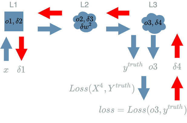
This is where thinks get complicated because we have to compute the impacts of the weights on the $ Loss $ function. Yet, computing these impacts is not straightforward: they directly depend on the learning flow of “future” $ layers $. This is the principal role of the backward pass: use the reverse order of the $ layers $ in order to compute the different learning flow.
In the previous article, we saw one last detail. Focusing on the backward pass of some $ L^{k} $ $ layer $ with some weights in it, we can compute the impacts of its weights right inside its backward pass:
- having access to the “future” learning flow of $ L^{k+1} $ ($ \delta^{k+1}) $ allows to compute $ \delta^{k} $: this is the impacts of the inputs of $ L^{k} $ on the $ Loss $ function. This is the primary goal of the backward pass.
- having access to $ \delta^{k+1} $ allows to compute $ \delta w^k $: this is the impacts of the weights of $ L^{k} $ on the $ Loss $ function. This is the secondary goal of the backward pass but the primary goal of the learning process itself !
Now, let us get back to our learning process.
What we have…
- a dataset containing (data input, data output):
- we want to run a $ model $ on the data input in order to produce results
- we want to confront the results produced against the expectations given by the data output
-
a $ model $ function, structured as a graph of $ layers $ which tries to understand the data input
- a $ Loss $ function which systematically compares the results of $ model $ to the expectations
What we do…
In the first paragraph, we saw that the learning process of a deep learning $ model $ happens during the training phase.
Through the different articles: Loss function, backward pass and weights, we explored the different parts that were specific to this training phase.
We are now able to give the different steps of the training phase in the right order:
- pick one data input in the dataset
- run the forward pass for the $ model $ on this data input
- use the $ Loss $ function to compute the error between the result produced by the $ model $ and the expectation given by the data output
- run the backward pass to compute:
- the learning flow
- the $ derivative $ of the $ Loss $ function according to $ W $
- update the weights of $ model $
As we want our $ model $ to learn on every data of our dataset we will repeat the previous points until we have “picked” every data input of our dataset.
The Gradient Descent Algorithm
In the previous article, we saw that in order to update the weights we use a formula with a direction of update: $ -\delta w $ and a length of update: $ \alpha $ which we called the learning rate.
We mentioned how this learning rate had to be very small in order not to break our local “prediction” of the $ Loss(model(X), Y^{truth}) $ function evaluated on (data input, data output).
The remaining problem is that if we use a very small learning rate, it means that after each weights update, the $ model $ will not learn a lot.
This is the reason why we repeat the whole process several times in order that many “small understanding steps” converge to a global understanding of the whole dataset.
This is the gradient descent algorithm which mainly consists in repeating what we already know:
- pick one data input in the dataset
- run the forward pass for the $ model $ on this data input
- use the $ Loss $ function to compute the error between the result produced by the $ model $ and the expectation given by the data output
- run the backward pass to compute:
- the learning flow
- the $ derivative $ of the $ Loss $ function according to $ W $
- update the weights of $ model $
As before, we do it for all data input in the dataset, we call it an epoch.
What changes now is that we continue running these points during several more epochs. That way, we have many “small understanding steps” for every data input of our dataset which helps alleviate the small learning rate.
Where does gradient descent name comes from ?
From the weights update formula of the last article:
\[\hat{w} = w - \alpha . \frac{\partial Loss}{\partial W}(x, y^{truth})\]For multivariate functions (function with multiple variables), the $ \frac{\partial Loss}{\partial W} $ is called the gradient.
It is a gradient descent because we follow the direction of $ -\frac{\partial Loss}{\partial W} $ to update the weights. And from what we saw in the paragraph “The derivative of Loss according to W” in the last article, it corresponds to the $ x $ axis direction where the tangent is descending.

Example: what we have…
We use the same example as in the previous articles. Let us recap the formula we have found for our $ model $ example.
Data
Same data as in the first article.
| data input | data output (expectation) |
|---|---|
| (100 broccoli, 2000 Tagada strawberries, 100 workout hours) | (bad shape) |
| (200 broccoli, 0 Tagada strawberries, 0 workout hours) | (good shape) |
| (0 broccoli, 2000 Tagada strawberries, 3 000 workout hours) | (good shape) |
Model
Same $ model $ as in the previous article.
\[\begin{align} L1(X^1) &= X^1 & \text{ with } X^1 = (X^1_1, X^1_2, X^1_3) \\ L2(X^2, W^2) &= W^2 . X^2 & \text{ with } X^2 = (X^2_1, X^2_2, X^2_3) \\ & & \text{ and } W^2 = (W^2_1, W^2_2, W^2_3) \\ &= W^2_1 . X^2_1 + W^2_2 . X^2_2 + W^2_3 . X^2_3 \\ L3(X^3) &= X^3 \text{ if } X^3 \geq 0 \text{ else } 0 \\ \\ model(X) &= L3(L2(L1(X))) & \text{ with } X = (X_1, X_2, X_3) \\ Loss(X^4, Y^{truth}) &= \frac{1}{2} (X^4 - Y^{truth})^2 \end{align}\]With the values of $ w^2 $:
\[w^2 = (\frac{1}{200}, -\frac{3 000}{11 600 000}, \frac{1}{5 800})\]Run the Forward Pass
| $ x $ | $ o1 = L1(x) $ | $ o2 = L2(o1) $ | $ o3 = L3(o2) $ |
|---|---|---|---|
| (100, 2000, 100) | (100, 2000, 100) | (0) | (0) |
| (200, 0, 0) | (200, 0, 0) | (1) | (1) |
| (0, 2000, 3 000) | (0, 2000, 3 000) | (0) | (0) |
| $ o3 = model(x) $ | $ y^{truth} $ | $ loss = Loss(o3, y^{truth}) $ | correct ? |
|---|---|---|---|
| (0) | (0) | (0) |  |
| (1) | (1) | (0) | |
| (0) | (1) | (0.5) |  |
Run the Backward Pass
Update the Weights
We have to use the update formula for $ w^2 $ :
\[\boxed{\hat{w^2} = w^2 - \alpha . \delta w^2}\]Example: what we do…
Let us run the training phase with a very small learning rate $ \alpha = 10^{-7} $. The $ model $ has to learn on each data input of our dataset. Thus we will run the training phase on our 3 data input: this will be one epoch of the gradient descent algorithm.
Run the Training Phase on the 1st Data Input
-
pick data input: $ x = (100, 2000, 100) $
-
run the forward pass:
\[\begin{align} o3 &= model(x) \\ &= model((100, 2000, 100)) \\ &= (0) \end{align}\] -
compute $ loss $
\[\begin{align} loss &= Loss(o3, y^{truth}) \\ &= (0) \end{align}\] -
run the backward pass:
\[\begin{align} \delta 4 &= o3 - y^{truth} \\ &= (0) - (0) \\ &= (0) \\ \delta 3 &= \delta 4 \text{ if } o2 \geq 0 \text{ else } 0 \\ &= (0) \text{ if } (0) \geq 0 \text{ else } 0 \\ &= (0) \\ \delta 2 &= \delta 3 * w2 \text{ with } w^2 = (\frac{1}{200}, -\frac{3 000}{11 600 000}, \frac{1}{5 800}) \\ &= (0) * (\frac{1}{200}, -\frac{3 000}{11 600 000}, \frac{1}{5 800}) \\ &= (0, 0, 0) \\ \delta w^2 &= \delta 3 * o1 \\ &= (0) * (100, 2000, 100) \\ &= (0, 0, 0) \\ \delta 1 &= \delta 2 \\ &= (0, 0, 0) \end{align}\] -
update the weights of $ model $
\[\begin{align} \hat{w^2} &= w^2 - \alpha . \delta w^2 \\ &= (\frac{1}{200}, -\frac{3 000}{11 600 000}, \frac{1}{5 800}) - 10^{-7} * (0, 0, 0) \\ &= (\frac{1}{200}, -\frac{3 000}{11 600 000}, \frac{1}{5 800}) \end{align}\]
It appears the new value for $ w^2 $ is still the same ! This is no wonder as for this first data input: $ loss = 0 $. This $ loss $ value is typical for a $ model $ that has already produced the right result and has nothing to learn.
Run the Training Phase on the 2nd Data Input
-
pick data input: $ x = (200, 0, 0) $
-
run the forward pass: [1]
\[\begin{align} o3 &= model(x) \\ &= model((200, 0, 0)) \\ &= (1) \end{align}\] -
compute $ loss $
\[\begin{align} loss &= Loss(o3, y^{truth}) \\ &= (0) \end{align}\] -
run the backward pass:
\[\begin{align} \delta 4 &= o3 - y^{truth} \\ &= (1) - (1) \\ &= (0) \\ \delta 3 &= \delta 4 \text{ if } o2 \geq 0 \text{ else } 0 \\ &= (0) \text{ if } (1) \geq 0 \text{ else } 0 \\ &= (0) \\ \delta 2 &= \delta 3 * w2 \text{ with } w^2 = (\frac{1}{200}, -\frac{3 000}{11 600 000}, \frac{1}{5 800}) \\ &= (0) * (\frac{1}{200}, -\frac{3 000}{11 600 000}, \frac{1}{5 800}) \\ &= (0, 0, 0) \\ \delta w^2 &= \delta 3 * o1 \\ &= (0) * (200, 0, 0) \\ &= (0, 0, 0) \\ \delta 1 &= \delta 2 \\ &= (0, 0, 0) \end{align}\] -
update the weights of $ model $
\[\begin{align} \hat{w^2} &= w^2 - \alpha . \delta w^2 \\ &= (\frac{1}{200}, -\frac{3 000}{11 600 000}, \frac{1}{5 800}) - 10^{-7} * (0, 0, 0) \\ &= (\frac{1}{200}, -\frac{3 000}{11 600 000}, \frac{1}{5 800}) \end{align}\]
Once more, the new value for $ w^2 $ has not changed. The same remark as before applies: $ loss = 0 $ means the $ model $ already produced the right result for this second data input and has nothing to learn.
Run the Training Phase on the 3rd Data Input
-
pick data input: $ x = (0, 2000, 3 000) $
-
run the forward pass: [1]
\[\begin{align} o3 &= model(x) \\ &= model((0, 2000, 3 000)) \\ &= (0) \end{align}\] -
compute $ loss $
\[\begin{align} loss &= Loss(o3, y^{truth}) \\ &= (0.5) \end{align}\] -
run the backward pass:
\[\begin{align} \delta 4 &= o3 - y^{truth} \\ &= (0) - (1) \\ &= (-1) \\ \delta 3 &= \delta 4 \text{ if } o2 \geq 0 \text{ else } 0 \\ &= (-1) \text{ if } (0) \geq 0 \text{ else } 0 \\ &= (-1) \\ \delta 2 &= \delta 3 * w2 \text{ with } w^2 = (\frac{1}{200}, -\frac{3 000}{11 600 000}, \frac{1}{5 800}) \\ &= (-1) * (\frac{1}{200}, -\frac{3 000}{11 600 000}, \frac{1}{5 800}) \\ &= -(\frac{1}{200}, -\frac{3 000}{11 600 000}, \frac{1}{5 800}) \\ \delta w^2 &= \delta 3 * o1 \\ &= (-1) * (0, 2000, 3 000) \\ &= -(0, 2000, 3 000) \\ \delta 1 &= \delta 2 \\ &= -(\frac{1}{200}, -\frac{3 000}{11 600 000}, \frac{1}{5 800}) \end{align}\] -
update the weights of $ model $
\[\begin{align} \hat{w^2} &= w^2 - \alpha . \delta w^2 \\ &= (\frac{1}{200}, -\frac{3 000}{11 600 000}, \frac{1}{5 800}) - 10^{-7} * (-(0, 2000, 3 000)) \\ &= (\frac{1}{200}, -\frac{3 000}{11 600 000}, \frac{1}{5 800}) + (0, 0.0002, 0.0003) \\ &= (\frac{1}{200}, 0.0002 - \frac{3 000}{11 600 000}, 0.0003 + \frac{1}{5 800}) \end{align}\]Let us keep in mind the new values we computed for $ w^2 $:
\[\boxed{w^2 = (\frac{1}{200}, 0.0002 - \frac{3 000}{11 600 000}, 0.0003 + \frac{1}{5 800})}\]
We have just run one epoch of the gradient descent algorithm on our whole dataset. Let us stop our algorithm now and check the new results when we run a new forward pass on every data input of our dataset.
Run a New Forward Pass
| $ x $ | $ o1 = L1(x) $ | $ o2 = L2(o1) $ | $ o3 = L3(o2) $ |
|---|---|---|---|
| (100, 2000, 100) | (100, 2000, 100) | (0.43) | (0.43) |
| (200, 0, 0) | (200, 0, 0) | (1) | (1) |
| (0, 2000, 3 000) | (0, 2000, 3 000) | (1.3) | (1.3) |
We see that our new results do not come along with (0) => (bad shape) and (1) => (good shape). We will add a new column in order to show the result that is aligned with (0) or (1) in order to compare with the expectations. Let us use a threshold to make the decision:
- values < 0.5 will be transformed to 0,
- values $ \geq $ 0.5 will be transformed to 1
Now we have:
| $ x $ | $ o3 = model(x) $ | $ result $ |
|---|---|---|
| (100, 2000, 100) | (0.43) | (0) |
| (200, 0, 0) | (1) | (1) |
| (0, 2000, 3 000) | (1.3) | (1) |
We are now able to compare $ result $ with $ y^{truth} $. In order to have a more objective indicator we still compute $ loss $ with the real outputs of our $ model $: $ o3 $
| $ o3 = model(x) $ | $ result $ | $ y^{truth} $ | $ loss = Loss(o3, y^{truth}) $ | correct ? |
|---|---|---|---|---|
| (0.43) | (0) | (0) | (0.092) | |
| (1) | (1) | (1) | (0) | |
| (1.3) | (1) | (1) | (0.045) | |
We observe that the $ result $ is now aligned with the expectation $ y^{truth} $ on the 3 data input !
The $ model $ has well learnt. Still, the $ loss $ for the first data input has increased. In the past its $ loss $
was 0 and now 0.092. This shows that any learning made on one data input may affect the understanding of
other data input ![]()
Conclusion
In this article we run the whole gradient descent algorithm and saw the learning process in action. We saw the gradient descent name comes from the direction followed to update the weights.
We run only one epoch of the algorithm and saw the weights’ updates have slightly degraded some results that were perfect in the original state. We could have run a second epoch to see how the situation evolves. Rather than that we will talk about an upgrade to the current algorithm. This upgrade will help stabilize learning at each iteration. Let us go to the next article !
Note that it is a “coincidence” that our $ model $ did not learn anything on the previous data input. If it had learnt anything, we would have updated the $ w^2 $ value and the results of the forward pass would have differed from the values that we computed in the past. This is the reason why we should keep in mind to run the forward pass on one data input at a time when the goal is to update weights.