Inside the Model
Introduction
In the previous article, we mentioned the prominent part the deep learning $ model $ plays in the learning.
In this article we will explore the $ model $ structure further.
The Layers
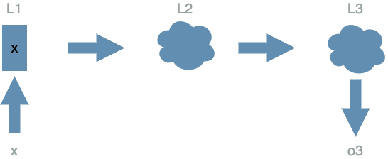
Without any further ado, here is what a typical deep learning $ model $ looks like:
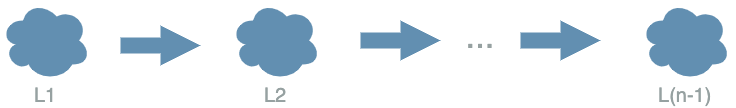
The two main components are the clouds and the arrows. For now we do not know what is in the clouds, just that we will call them $ layers $ ($ L1 $, $ L2 $, …). But we can clearly see what the arrows imply…
The Forward Pass
The arrows imply a sequential order, letting the information flow pass through the different $ layers $.
If we recall the paragraph “Run a model” in the previous article, we saw that if we consider a $ model $ function, we could evaluate it on some values to produce results.
Now, we have a more precise structure for this $ model $ function, as a sequential order of $ inner \text{ } functions $ (the clouds), each depending on its previous function. So that if $ layer $ $ L^k $ depends on $ X^k $ and $ layer $ $ L^{k+1} $ depends on $ X^{k+1} $:
\[\boxed{X^{k+1} = L^k(X^k)}\]The $ layer $ results are called representations. The output representations of any layer are the input of their immediate following $ layer $ in the sequential order.
While going deeper in the $ layers $, the representations will contain an understanding more complex and more abstract of the input data.
This is the goal of deep learning: considering the representations of the last $ layer $, we want it to have the best understanding of the input data possible.
While they seem abstract for the moment, these representations will be more precise in the linear function article. But we have some articles to read before that…
Example
Data
Same data as in the previous article.
| data input | data output (expectation) |
|---|---|
| (100 broccoli, 2000 Tagada strawberries, 100 workout hours) | (bad shape) |
| (200 broccoli, 0 Tagada strawberries, 0 workout hours) | (good shape) |
| (0 broccoli, 2000 Tagada strawberries, 3 000 workout hours) | (good shape) |
Model
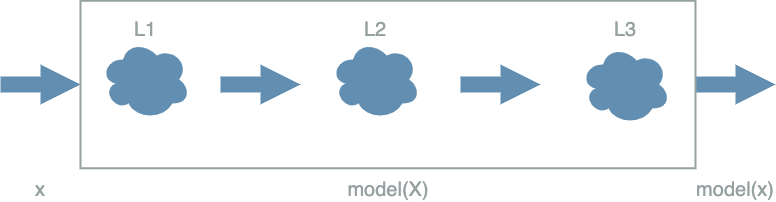
We assume we have a $ model $ containing only 3 $ layers $:
Let us use:
\[\begin{align} L1(X^1) &= X^1 & \text{ with } X^1 = (X^1_1, X^1_2, X^1_3) \\ L2(X^2) &= \frac{1}{200} X^2_1 - \frac{3 000}{11 600 000} X^2_2 + \frac{1}{5 800} X^2_3 & \text{ with } X^2 = (X^2_1, X^2_2, X^2_3) \\ L3(X^3) &= X^3 \text{ if } X^3 \geq 0 \text{ else } 0 \\ \\ model(X) &= L3(L2(L1(X))) & \text{ with } X = (X_1, X_2, X_3) \end{align}\]We verify that:
- $ X $ is a vector with 3 numbers: $ X_1 $ is the variable for broccoli, $ X_2 $ is the variable for Tagada strawberries, $ X_3 $ is the variable for workout hours
- $ model(X) $ is a simple number
We have built a $ model $ that is composed of 3 layers ($ L1 $, $ L2 $, $ L3 $).
Run the Forward Pass
Instead of using $ model(X) $ directly as in the previous article. We now have to apply the forward pass, storing every intermediate results.
- first we have to evaluate $ L1 $ on $ x $ as $ L1 $ is our first layer => L1 produces a new output, let $ o1 $ be it
- then we evaluate $ L2 $ on the result of $ L1 $ which is $ o1 $ => L2 produces a new output, let $ o2 $ be it
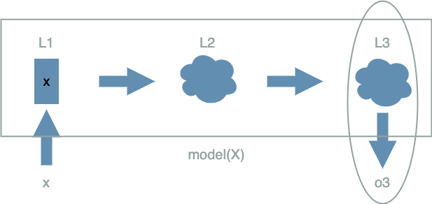
- finally we evaluate $ L3 $ on the result of $ L2 $ which is $ o2 $ => L3 produces a new output, let $ o3 $ be it
It appears that: \(model(x) = o3\)
Here are the different results on the data:
| $ x $ | $ o1 = L1(x) $ |
|---|---|
| (100, 2000, 100) | (100, 2000, 100) |
| (200, 0, 0) | (200, 0, 0) |
| (0, 2000, 3 000) | (0, 2000, 3 000) |
| $ o1 $ | $ o2 = L2(o1) $ |
|---|---|
| (100, 2000, 100) | (0) |
| (200, 0, 0) | (1) |
| (0, 2000, 3 000) | (0) |
| $ o2 $ | $ o3 = L3(o2) $ |
|---|---|
| (0) | (0) |
| (1) | (1) |
| (0) | (0) |
Finally we summarize these results:
| $ x $ | expected result | $ o3 = model(x) $ | correct ? |
|---|---|---|---|
| (100, 2000, 100) | (bad shape) | (0) => (bad shape) |  |
| (200, 0, 0) | (good shape) | (1) => (good shape) | |
| (0, 2000, 3 000) | (good shape) | (0) => (bad shape) |  |
We observe that although we have changed the structure of $ model $ compared to the
previous article, we still get exactly the same results.
Which is in fact normal: although we changed its structure, we have built the same “global” function as in the
previous article ![]()
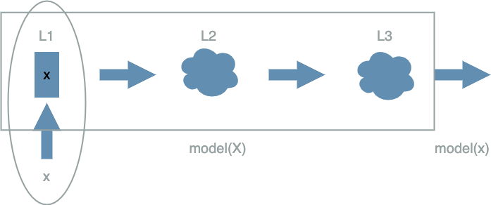
The Input Layer
The input layer is the first layer of the $ model $. It is special in that it does not need the output of its previous layer in the forward pass order to produce an output.
When the developer wants to run the $ model $ on some $ x $ data, the developer will in fact give
$ x $ directly to the input layer. In that way it does not even need to produce a value,
as it already owns this data.
Note as in the example, the input layer was just outputting its input without any modification: $ L1(X^1) = X^1 $.
The Output Layer
The output layer is the last layer of the $ model $. It is special in that its value is not used by any other layers.
Its value is in fact the final output of the $ model $ and this is the value that we want to compare to the data output expectation.
The Layer in General
As we saw in the example, each $ layer $ is a mathematical function that depends on some variable which will receive the output of its previous $ layer $. For example $ L2 $ depends on $ X^2 $. During the forward pass, we need to wait for $ L1 $ to produce $ o1 $ so that $ L2 $ can use it to produce $ o2 $: $ o2 = L2(o1) $.
When we run a $ model $ on some data we want to produce the output of its output layer (see the output layer).
Using the example $ model $, running $ model $ on $ x $ is about producing the result of $ L3 $ on the output of $ L2 $. The output of $ L2 $ is itself the result of $ L2 $ computed on the output of $ L1 $. The output of $ L1 $ has been given by the developer (see the input layer).
We can put it as:
\[model(x) = L3(L2(L1(x)))\]Conclusion
In this article, we saw that the global structure of a deep learning $ model $ is in fact an ordered graph of $ layers $ as in the following schema:
In a later chapter we will discuss the different forms of the $ layers $. But before that, we will talk about the $ Loss function $ in the next article.