The Loss function
Introduction
In the previous article, we explored the generic structure of the deep learning $ model $: an ordered graph of $ layers $.
In this article we will talk about the $ Loss $ function which is the starting point of the learning process.
The Learning Process
In the paragraph “Training, Inferring” of the first article, we talked about the training phase and the inferring phase. It is no surprise that the learning process in deep learning happens during the training phase. We will concentrate on it.
During this phase we run the forward pass (see the previous article). Then we are able to get the final results of our $ model $ thanks to its output layer.
In the different “Example” paragraphs, two special values were comparable:
- $ o3 $: the output layer result when we run the $ model $ on the data input.
- the expected result which is the data output.
We compared $ o3 $ to the expected result and two situations occurred: $ o3 = expectation $ or $ o3 \neq expectation $.
We are now looking for a systematic way of telling the $ model $: this result is right, that result is wrong.
The Loss Function
The systematic way of telling the $ model $ what is right or wrong is the $ Loss $ function.
This $ Loss $ function is defined by the developer. It is a function of two variables: $ X $ (as every $ layer $) and $ Y^{truth} $ (the expectation, see the first article).
The $ X $ variable will receive the result of the output layer whereas $ Y^{truth} $ will receive the expectation given by the data output. Hence, the $ Loss $ function will be able to systematically compare them both.
This also implies the $ Loss $ function will be called after the output layer:
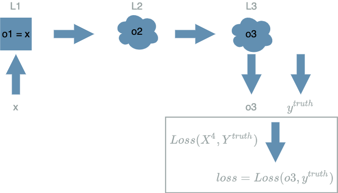
We will note $ loss $ when we evaluate the $ Loss $ function on some values. A standard property we want for the $ Loss $ function is that $ loss \geq 0 $. The final goal of the learning process is that $ loss = 0 $ on every data of the dataset. Said differently we want to minimize the $ Loss $ function.
The Derivative Operator
The $ derivative $ operator is what makes the learning process possible. For an $ f $ function depending on $ X $, we can apply the $ derivative $ operator on $ f $ according to $ X $. That way, we build a new function, noted $ \frac{df}{dX} $. This new function can be evaluated on some value, for example $ x $:
\[\frac{df}{dX}(x) = \lim_{h \to 0} \frac{f(x + h) - f(x)}{h}\]We use the $ \frac{d}{dX} $ notation to apply the operator on a function with only one variable. We will prefer the notation $ \frac{\partial}{\partial X} $ because our functions have potentially several variables.
There are two very interesting properties of this $ derivative $ operator.
- It builds kind of a prediction at the point $ x $.
- From a explicit formula for $ f $, we are able to compute an explicit formula for $ \frac{\partial f}{\partial X} $.
The two points are incredibly powerful.
-
When we run the forward pass we cannot apply our $ model $ to an infinite number of data: we have just a finite number of them. If we consider a well known point ($ x $, $ f(x) $), the $ derivative $ operator links a “theoretical” small move from $ x $ in the $ X $ variable direction, let say $ \hat{x} = x + h $, to the prediction of the new value $ f(\hat{x}) $. This new point ($ \hat{x} $, $ f(\hat{x}) $) did not exist in the dataset. Said differently, we know the impact of $ X $ on $ f $.
-
The $ layer $ structure of our $ model $ will help us compute explicit formulas for the different $ derivatives $ we are looking for thanks to some formulas we learnt at school. What you might have guessed is actually happening now: we are going to apply the $ derivative $ operator to the $ Loss $ function. That way, we will be able to compute the impact of any variable in the $ model $ on the $ Loss $ function. Said differently, we will be able to predict how a slight modification of any variable in the $ model $ will affect the $ loss $ final value. We will see why this is interesting in a later article.
More practically we will keep in mind that applying the $ derivative $ operator on $ f $ according to $ X $ gives a new function for which we can compute an explicit formula:
\[\begin{align} derivative \text{ }f \text{ according to } X &= \frac{\partial}{\partial X}(f(X)) \\ &= \frac{\partial f}{\partial X} \end{align}\]Once we get the explicit formula, we can evaluate this function on $ x $:
\[\boxed{\frac{\partial f}{\partial X}(x)}\]The Derivative of the Loss Function
What we have for the moment is:
- a $ model $ function which depends on $ X $
- running the forward pass on $ x $ value for $ X $ produces $ model(x) $
- evaluating $ Loss(model(x), y^{truth}) $ decides whether $ model(x) $ is right or wrong
We can already compute to what extent the variable $ X $ in the $ model $ is responsible for the errors that are highlighted by the $ Loss $ function. For the moment we do not really know why this is useful (we will talk about it in this article).
Thanks to the last paragraph, we know we have to compute the $ derivative $ function of $ Loss $ according to $ X $:
\[\begin{align} derivative \text{ of }Loss \text{ according to } X &= \frac{\partial}{\partial X}(Loss(model(X), Y^{truth})) \\ &= \frac{\partial Loss}{\partial X} \end{align}\]Let us keep in mind this notation:
\[\boxed{\frac{\partial Loss}{\partial X}}\]Then we also know that we have to evaluate this function. What values should we choose for this evaluation ?
We want to evaluate $ \frac{\partial Loss}{\partial X} $ on the same values $ x $ and $ y^{truth} $ that produced the errors for the function $ Loss(model(X), Y^{truth}) $, with $ x $ the data that was taken from our dataset and $ y^{truth} $ the associated expectation. We will call this final result $ \delta $:
\[\boxed{\delta = \frac{\partial Loss}{\partial X}(x, y^{truth})}\]We could paraphrase the formula as: we want to know to what extent the variable $ X $ causes an error when the $ Loss(model(X), Y^{truth}) $ function is evaluated on $ x $ and $ y^{truth} $ and we slightly disturb $ x $.
Another way to put it: we want to know the impact of $ X $ on the $ Loss $ function.
Example
Data
Same data as in the first article.
| data input | data output (expectation) |
|---|---|
| (100 broccoli, 2000 Tagada strawberries, 100 workout hours) | (bad shape) |
| (200 broccoli, 0 Tagada strawberries, 0 workout hours) | (good shape) |
| (0 broccoli, 2000 Tagada strawberries, 3 000 workout hours) | (good shape) |
Model
We assume we have a $ model $ containing only 3 $ layers $. We also add a $ Loss $ function:
Let us use:
\[\begin{align} L1(X^1) &= X^1 & \text{ with } X^1 = (X^1_1, X^1_2, X^1_3) \\ L2(X^2) &= \frac{1}{200} X^2_1 - \frac{3 000}{11 600 000} X^2_2 + \frac{1}{5 800} X^2_3 & \text{ with } X^2 = (X^2_1, X^2_2, X^2_3) \\ L3(X^3) &= X^3 \text{ if } X^3 \geq 0 \text{ else } 0 \\ \\ model(X) &= L3(L2(L1(X))) & \text{ with } X = (X_1, X_2, X_3) \\ Loss(X^4, Y^{truth}) &= \frac{1}{2} (X^4 - Y^{truth})^2 \end{align}\]We verify that:
- $ X $ is a vector with 3 numbers: $ X_1 $ is the variable for broccoli, $ X_2 $ is the variable for Tagada strawberries, $ X_3 $ is the variable for workout hours
- $ model(X) $ is a simple number
- $ Loss $ is a loss function that depends on $ X^4 $ and $ Y^{truth} $, $ X^4 $ receiving the value of the output layer of $ model $.
We have built a $ model $ that is composed of 3 layers ($ L1 $, $ L2 $, $ L3 $).
Run the Forward Pass
First of all let us run the forward pass:
| $ x $ | $ o1 = L1(x) $ |
|---|---|
| (100, 2000, 100) | (100, 2000, 100) |
| (200, 0, 0) | (200, 0, 0) |
| (0, 2000, 3 000) | (0, 2000, 3 000) |
| $ o1 $ | $ o2 = L2(o1) $ |
|---|---|
| (100, 2000, 100) | (0) |
| (200, 0, 0) | (1) |
| (0, 2000, 3 000) | (0) |
| $ o2 $ | $ o3 = L3(o2) $ |
|---|---|
| (0) | (0) |
| (1) | (1) |
| (0) | (0) |
| $ o3 = model(x) $ | $ y^{truth} $ = expected result | $ loss = Loss(o3, y^{truth}) $ | correct ? |
|---|---|---|---|
| (0) | (0) | (0) |  |
| (1) | (1) | (0) | |
| (0) | (1) | (0.5) |  |
We observe that the value of $ loss(o3, y^{truth}) $ is 0 when there is no error comparing $ o3 $ with $ y^{truth} $ and is higher than 0 when there is an error . The $ loss $ is indeed an indicator of the error of the results produced by the $ model $ function.
Going Further
 mathematically shy people should jump to the conlusion
Even if we do not really know why this is useful for the moment, let us try to compute the explicit formula for the $ derivative $ function of our $ Loss $ function according to $ X $ in our $ model $:
\[\frac{\partial Loss}{\partial X}\]Do not forget our $ model $ is composed of several $ layers $. Each of these $ layers $ is responsible for the error highlighted by the $ Loss $ function. So we must compute the derivative for each of their dependency variables:
\[\frac{\partial Loss}{\partial X^1} \text{, } \frac{\partial Loss}{\partial X^2} \text{, } \frac{\partial Loss}{\partial X^3} \text{, and } \frac{\partial Loss}{\partial X^4}\]These different $ derivative $ functions won’t be as easy to compute. The easiest is the last one because we have:
\[Loss(X^4, Y^{truth}) = \frac{1}{2} (X^4 - Y^{truth})^2\]Thus, we can compute an explicit formula for the $ derivative $ function of $ Loss $ according to $ X^4 $:
\[\begin{align} \frac{\partial Loss}{\partial X^4} & = \frac{\partial (\frac{1}{2} (X^4 - Y^{truth})^2)}{\partial X^4}\\ & = 2 * \frac{1}{2} * (X^4 - Y^{truth}) \\ &= X^4 - Y^{truth} \\ \end{align}\]We can now evaluate this function on the values that have produced $ loss = Loss(o3, y^{truth}) $, let $ \delta 4 $ be this result:
\[\begin{align} \delta 4 &= \frac{\partial Loss}{\partial X^4}(o3, y^{truth}) \\ &= X^4 - Y^{truth} \text{ evaluated on } (o3, y^{truth}) \\ &= o3 - y^{truth} \end{align}\]Let us keep in mind that we have computed:
\[\boxed{\delta 4 = o3 - y^{truth}}\]Back to the other $ derivative $ functions, what is the problem now ? Let us look at:
\[\frac{\partial Loss}{\partial X^3}\]We need to find to what extent the variable $ X^3 $ causes an error in the $ Loss $ function. We know that:
\[\begin{align} L3(X^3) &= X^3 \text{ if } X^3 \geq 0 \text{ else } 0 \\ Loss(X^4, Y^{truth}) &= \frac{1}{2} (X^4 - Y^{truth})^2 \\ \end{align}\]The question that may arise is: $ X^3 $ is defined in $ L3 $, not in the $ Loss $ function, so how could it be responsible for the error highlighted by the $ Loss $ function ?
This is due to the structure in $ layers $ of our $ model $. Changing the value for $ X^3 $ impacts the $ layers $ that use $ X^3 $ directly ($ L3 $) or indirectly ($ L4 $, $ L5 $, …, $ Loss $) . [1]
This is the beauty of the $ derivative $: from a single $ loss $ result, being able to find the different culprits and to what extent they are responsible for the final error through a chain of $ layers $ (we will talk about this chaining aspect in the next article).

Conclusion
In this article, we saw the importance of the $ Loss $ function in order to set what results of $ model $ are right or wrong.
We also saw the $ derivative $ of $ Loss $ according to $ X $ that allows to measure to what extent $ X $ is responsible for the final error when we slightly disturb $ x $:
\[\boxed{\delta = \frac{\partial Loss}{\partial X}(x, y^{truth})}\]We were able to compute this $ derivative $ function according to the final variable but not
according to the inner variables.
We will need to see how it works for the inner variables
in the next article ![]()
In fact this means the $ Loss $ function depends on more variables than just $ X^4 $ and $ Y^{truth} $. Talking about $ Loss(X^1, X^2, X^3, X^4, Y^{truth}) $ would be more precise. This also applies for every $ layer $: $ L3(X^1, X^2, X^3) $, $ L2(X^1, X^2) $ and $ L1(X^1) $.
For our comfort, we will keep the notation with direct variables: $ Loss(X^4, Y^{truth}) $, $ L3(X^3) $, $ L2(X^2) $ and $ L1(X^1) $. ↑