The Weights
Introduction
In the previous article, we computed the learning flow for each $ layer $ in our $ model $.
In this article we will explore the reason for these computations: update the model’s weights.
But before that, let us introduce the $ model $’s weights, responsible for the learning process ![]()
The Model’s Weights
We have spoken about them for a long time now. But what are they ?
Well, just another variable. We already saw a few of them: $ X $ the generic input variable of a $ layer $. $ Y^{truth} $ a variable used in the $ Loss $ function to receive the expectations. Here we introduce $ W $, the weights. They are the essential part for the $ model $ to be trained.
In fact, if the weights were really just another variable, we could have incorporated them in the $ X $ generic variable (which is itself potentially multi dimensional). But there are two main differences between $ X $ and $ W $:
- $ W $ does not receive its value from the previous $ layer $ such as $ X $
- $ W $ values do not come from the data but are given by the developer
Understanding the real effect of weights on a $ model $ is not that easy. We will speak about it longer in later articles. The principal property that is interesting about them is that they are the only moving part of the $ model $ the developer has access to.
What does this mean ? Let us consider the small scenario:
- We pick one data in a dataset and compute a forward pass on it, we produce some results.
- We pick the exact same data in the dataset and compute a forward pass on it again, we produce the exact same results.
But as our goal is to learn from our failures we will use the weights in order to change that state:
- We pick the previous data in the dataset, we compute a forward pass to produce some results
- We update the weights values in order to learn
- We pick the exact same data in the dataset and compute a forward pass on it, the result we be different now.
For now, none of the $ model $ functions we used in the different examples had weights. In order to see how to deal with them, we will modify some parts of our example to add some of them. Note that it is not necessary to use them in every $ layer $ (we will talk about that longer in later articles).
So for each $ layer $ $ L^k $ that declares weights, we have two dependencies: $ X^k $ and $ W^k $. And for each $ layer $ $ L^i $ that does not declare weights, one dependency: $ X^i $.
The Learning Process
We have just introduced the weights and said the developer can change their values. In this paragraph we elaborate on the special moment when the developer updates them, the core of the learning process.
There is one property that makes $ W $ very special: sometimes it will be a variable and sometimes not. That is the main reason of the existence of the training phase we introduced in the first article.
During the training phase, $ W $ will be a variable and the developer will modify it so that the modifications help the $ model $ producing better results.
During the inferring phase, $ W $ won’t be a variable any more. It will stay at the last value it had during the training phase.
We hope that during the training phase the $ model $’s understanding of the data is getting better and better, so that this last value is the best that was learnt during the training phase.
What is important to keep in mind is that the weights have a meta role. They are at the junction between the developer and the $ model $. During the training phase, the developer actively updates the weights for the $ model $ to perform better. During the inferring phase, the developer passively waits for the $ model $ to produce new results.
The Derivative of Loss according to W
We have just accepted that the weights are a moving part of the $ model $ and that the developer has to update them to make the $ model $ stronger. But we do not know how to update them. The idea is to use the $ derivative $ operator.
In this article, we saw how “The derivative operator” enables us to compute the impact of any variable in $ model $ on the $ Loss $ function.
More specifically we start running the forward pass of our $ model $ on some $ x $ data in the dataset. Then we observe the results produced by the $ model $ and the $ loss $ value. The magical move is that we can slightly disturb any variable in our $ model $ and still be able to “predict” what the new $ loss $ value will be consequently to that change.
We choose to apply our magical move to the $ W $ variable: it means we can slightly disturb our weights and still be able to “predict” the new $ loss $ value. But in fact we do not really care about predicting this new value, what we really want is to minimize it…
This comes down to analysing the direction of modification for $ W $. We can disturb it positively or negatively. But as we know how to predict the new value of $ loss $ after the change, we know which direction, positive or negative, will bring a decrease in the $ loss $ value.
Let us have a look at a one dimensional example. Some years ago, we would hear our mathematical teacher say that: “the slope of the tangent line at a point on the function is equal to the derivative of the function at the same point”.

On this example the slope is positive (the tangent is “climbing the hill”). This means that if we add a small positive number to $ x $: let $ h $ be it, we can “predict” that $ f(x + h) > f(x) $ which is not what we want. But if we add the same number negatively we “predict” that: $ f(x - h) < f(x) $ which is exactly what we are looking for.
Note that if the slope had been negative (tangent is “running down the hill”) then we should have modified $ x $ with a positive small number in order for $ f $ to decrease: $ f(x + h) < f(x) $.
Anyway, this gives us the intuition that the right direction for the change is the opposit of the sign of the slope of the tangent. Said differently, the right direction is the $ x $ axis direction where the tangent is descending. But the slope of the tangent is itself the $ derivative $ of $ f $ according to $ X $ evaluated on $ x $ (remember our mathematical teacher).
Finally we will keep in mind that if we want to slightly disturb a variable of a function in order to minimize it, the small change has to be made in this direction:
\[-\frac{df}{dX}(x)\]Back to our weights we will follow the exact same direction to minimize our $ loss $ value evaluated on one $ x $ data of our dataset with the associated expectation $ y^{truth} $:
\[-\frac{\partial Loss}{\partial W}(x, y^{truth})\]As we mentioned in the “The derivative operator” paragraph of this article, we have to proceed in two steps:
- compute an explicit formula for $ \frac{\partial Loss}{\partial W} $
- evaluate the formula on $ x $ and $ y^{truth} $
We will call the final result $ \delta w $:
\[\boxed{\delta w = \frac{\partial Loss}{\partial W}(x, y^{truth})}\]We could paraphrase the formula as: we want to know to what extent the variable $ W $ causes an error in the $ model $ when the $ Loss $ function is evaluated on $ x $ and $ y^{truth} $ and we slightly disturb $ w $.
Another way to put it: we want to know the impact of $ W $ on the $ Loss $ function.
The Backward Pass for Weights
We are coming closer to justify the computations we made in the previous article. The whole thing is naturally linked to what we have just seen:
\[\delta w = \frac{\partial Loss}{\partial W}(x, y^{truth})\]As we mentioned, we first have to compute the explicit formula for $ \frac{\partial Loss}{\partial W} $ and then it will be easy to evaluate it. In order to compute the explicit formula we have to follow the exact same strategy we followed during the backward pass in the previous article.
Let us take some $ L^{k} $ $ layer $ declaring weights. $ L^{k} $ has two dependencies: $ X^{k} $ and $ W^{k} $. As in the backward pass we admit that we have already computed the “future” learning flow $ \delta^{k+1} $.
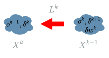
- The $ layer $ that directly uses $ W^{k} $ is $ L^{k} $ by definition: $ X^{k+1} = L^{k}(X^k, W^k) $.
- The link between $ X^{k+1} $ and $ Loss $ is the “future” learning flow: $ \delta^{k+1} $.
Using the chain rule (previous article) with $ z = Loss $ and $ y = L^{k} $, we have:
\[\frac{\partial Loss}{\partial W^{k}} = \frac{\partial Loss}{\partial L^{k}} . \frac{\partial L^{k}}{\partial W^{k}}\]Thanks to the forward pass we know that: $ X^{k+1} = L^{k}(X^{k}, W^{k}) $, so the formula becomes:
\[\boxed{\frac{\partial Loss}{\partial W^{k}} = \frac{\partial Loss}{X^{k+1}} . \frac{\partial L^{k}}{\partial W^{k}}}\]where $ \frac{\partial Loss}{X^{k+1}} $ is the “future” learning flow and $ \frac{\partial L^{k}}{\partial W^{k}} $ is a part we compute thanks to some formula we learnt at school.
This means that we are able to obtain the explicit formula for $ \frac{\partial Loss}{\partial W^{k}} $. Evaluating this function will finally give $ \delta w^k $…
This is the reason why we spent some time computing the learning flow. The learning flow is what propagates the knowledge of who did contribute to the final error and to what extent in the $ model $.
There is another remark: as soon as we have computed the learning flow for one particular $ L^{k+1} $ $ layer $, we can compute the learning flow for $ L^{k} $ (we already saw that in the backward pass). Now we see we may as well compute the impact of its weights on the $ Loss $ : $ \delta w^{k} $.
This means we may include the last operation in the backward pass.
For each $ L^{k} $ $ layer $ in the $ model $ in the reverse order of the forward pass do:
- compute the learning flow: $ \delta^k $
- compute the impact of its weights (if they exist) on the $ Loss $: $ \delta w^{k} $.

Update the Weights
In this paragraph, we have already spoken about the direction we must follow for our weights’ update:
\[-\delta w = -\frac{\partial Loss}{\partial W}(x, y^{truth})\]The missing piece is “how long can we go into that direction” ? The answer is really really not long because as we mentioned several times, the “prediction” we talked about in the “The derivative operator” paragraph of this article is very localized around the point where we evaluate the $ derivative $ function: hence the repeated mantra of “slight” modification…
Unfortunately there won’t be a more precise answer to that question. We will use a coefficient $ \alpha $, called the learning rate which will denote the length at which we follow the previous direction. But finding a good value for this coefficient is up to the developer, a meta-algorithm, belief or something else…
Now we are able to complete the formula to update the weights:
\[\hat{w} = w - \alpha . \frac{\partial Loss}{\partial W}(x, y^{truth})\]We recognize the direction of update: $ - \frac{\partial Loss}{\partial W}(x, y^{truth}) $, and the length of update: $ \alpha $.
We note $ \hat{w} $ to symbolize the new value that $ w $ will take at the end of the update.
And with the $ \delta w $ notation we have:
\[\boxed{\hat{w} = w - \alpha . \delta w}\]The Optimizer
Note that there exist plenty other ways to update the weights. Each have their advantages.
Anyway the most important part of them all is the direction of the update given by: $ -\delta w $. This direction is the core of the learning process and is computed during the backward pass.
In a framework where we would like to test the different ways to update the weights, the optimizer is the typical name for the component in charge of them.
If we take a look at this component, we should keep in mind that we “just” have to apply the formula, the different parts having been computed beforehand.
Example
We will use the same example as in the previous articles. But we will add some weights to our $ model $ in order to see how to update them. For now we just keep in mind that these weights are the only moving part of the $ model $ we can modify to make it better (see the first paragraph). We will explore their influence in later articles.
Data
Same data as in the first article.
| data input | data output (expectation) |
|---|---|
| (100 broccoli, 2000 Tagada strawberries, 100 workout hours) | (bad shape) |
| (200 broccoli, 0 Tagada strawberries, 0 workout hours) | (good shape) |
| (0 broccoli, 2000 Tagada strawberries, 3 000 workout hours) | (good shape) |
Model
We assume we have “nearly” the same $ model $ containing only 3 $ layers $ and a $ Loss $ function. But we modify $ L2 $ to add some weights. Previously we had:
\[L2(X^2) = \frac{1}{200} X^2_1 - \frac{3 000}{11 600 000} X^2_2 + \frac{1}{5 800} X^2_3 \text{ with } X^2 = (X^2_1, X^2_2, X^2_3)\]Now we change it to:
\[\begin{align} L2(X^2, W^2) &= W^2 . X^2 & \text{ with } X^2 = (X^2_1, X^2_2, X^2_3) \\ & & \text{ and } W^2 = (W^2_1, W^2_2, W^2_3) \\ &= W^2_1 . X^2_1 + W^2_2 . X^2_2 + W^2_3 . X^2_3 & \end{align}\]Here are all the $ layers $:
\[\begin{align} L1(X^1) &= X^1 & \text{ with } X^1 = (X^1_1, X^1_2, X^1_3) \\ L2(X^2, W^2) &= W^2 . X^2 & \text{ with } X^2 = (X^2_1, X^2_2, X^2_3) \\ & & \text{ and } W^2 = (W^2_1, W^2_2, W^2_3) \\ &= W^2_1 . X^2_1 + W^2_2 . X^2_2 + W^2_3 . X^2_3 \\ L3(X^3) &= X^3 \text{ if } X^3 \geq 0 \text{ else } 0 \\ \\ model(X) &= L3(L2(L1(X))) & \text{ with } X = (X_1, X_2, X_3) \\ Loss(X^4, Y^{truth}) &= \frac{1}{2} (X^4 - Y^{truth})^2 \end{align}\]We have indeed introduced weights in $ L2 $. But as any variable, we must pick some value in order to compute something. So let us say that the current values for $ W^2 $ are the same values we already used in the previous $ L2 $ function:
\[w^2 = (\frac{1}{200}, -\frac{3 000}{11 600 000}, \frac{1}{5 800})\]When we evaluate $ L2 $ on $ o1 $ output from $ L1 $ we have:
\[L2(o1, w^2) = w^2 * o1 = \frac{1}{200} * o^1_1 - \frac{3 000}{11 600 000} * o^1_2 + \frac{1}{5 800} * o^1_3\]which is exactly what we had when running the forward pass in the previous articles.
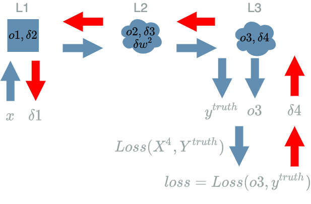
Run the Forward Pass
Same as in the Loss function article:
Run the Backward Pass for the Learning Flow
Let us keep in mind the results we already computed in the Loss function article and in the previous article.
\[\boxed{\delta 4 = o3 - y^{truth}}\] \[\boxed{\delta 3 = \delta 4 \text{ if } o2 \geq 0 \text{ else } 0}\] \[\delta 2 = \delta 3 * (\frac{1}{200}, -\frac{3 000}{11 600 000}, \frac{1}{5 800})\] \[\boxed{\delta 1 = \delta 2}\]But we keep in mind that:
\[\boxed{\delta 2 = \delta 3 . w2 \text{ with } w^2 = (\frac{1}{200}, -\frac{3 000}{11 600 000}, \frac{1}{5 800})}\] mathematically shy people should skip
Run the Backward Pass for the Weights
As mentioned in this paragraph we need to use the learning flow in order to compute the explicit formula for the $ derivative $ functions of $ Loss $ according to the weights.
Note that $ L2 $ is the only $ layer $ that declares weights in this $ model $. This is the reason why there is just one $ \delta w^2 $ in the diagram below.
We have to compute:
\[\boxed{\frac{\partial Loss}{\partial W^2}}\]As in the previous article, we are looking for a link between $ W^2 $ and $ Loss $. Once again the idea is to use the backward pass to link what we have already computed and what uses $ W^2 $: $ L2 $.
\[\begin{align} L2(X^2, W^2) &= W^2 . X^2 & \text{ with } X^2 = (X^2_1, X^2_2, X^2_3) \\ & & \text{ and } W^2 = (W^2_1, W^2_2, W^2_3) \\ &= W^2_1 . X^2_1 + W^2_2 . X^2_2 + W^2_3 . X^2_3 & \end{align}\]As previously, we remark that $ W^2 = (W^2_1, W^2_2, W^2_3) $. Thus, we have to compute the $ derivative $ functions of $ Loss $ according to each of them:
\[\frac{\partial Loss}{\partial W^2_1} \text{, } \frac{\partial Loss}{\partial W^2_2} \text{ and } \frac{\partial Loss}{\partial W^2_3}\]We are able to use the chain rule with $ z = Loss $ and $ y = L2 $, for $ W^2_1 $ the formula becomes:
\[\boxed{\frac{\partial Loss}{\partial W^2_1} = \frac{\partial Loss}{\partial L2} . \frac{\partial L2}{\partial W^2_1}}\]Thanks to the forward pass we know that $ X^3 = L2(X^2) $, so we have:
\[\frac{\partial Loss}{\partial L2} = \frac{\partial Loss}{\partial X^3} \text{ we recognize a learning flow !}\]and:
\[\begin{align} \frac{\partial L2}{\partial W^2_1} &= \frac{\partial (W^2_1 . X^2_1 + W^2_2 . X^2_2 + W^2_3 . X^2_3)}{\partial W^2_1} \text{ with the definition of } L2(X^2, W^2) \\ &= X^2_1 \end{align}\]Assembling those results:
\[\begin{align} \frac{\partial Loss}{\partial W^2_1} &= \frac{\partial Loss}{\partial L2} . \frac{\partial L2}{\partial W^2_1} \\ &= (\frac{\partial Loss}{\partial X^3}) * (X^2_1) \end{align}\]We can now evaluate this function on the values that have produced the final $ loss $, let $ \delta w^2_1 $ be this result:
\[\begin{align} \delta w^2_1 &= \frac{\partial Loss}{\partial W^2_1}(o1) \\ &= \frac{\partial Loss}{\partial X^3}(o2) * o1_1 \\ &= \delta 3 * o1_1 \end{align}\]We have found:
\[\delta w^2_1 = \frac{\partial Loss}{\partial W^2_1}(o1) = \delta 3 * o1_1\]We do the same to compute:
\[\delta w^2_2 = \frac{\partial Loss}{\partial W^2_2}(o1) = \delta 3 * o1_2\]and
\[\delta w^2_3 = \frac{\partial Loss}{\partial W^2_3}(o1) = \delta 3 * o1_3\]These 3 formulas can be summarized as:
\[\begin{align} \delta w^2 &= \frac{\partial Loss}{\partial W^2}(o1) \\ &= (\frac{\partial Loss}{\partial W^2_1}(o1), \frac{\partial Loss}{\partial W^2_2}(o1), \frac{\partial Loss}{\partial W^2_3}(o1)) \\ &= (\delta w^2_1, \delta w^2_2, \delta w^2_3) \\ &= (\delta 3 * o1_1, \delta 3 * o1_2, \delta 3 * o1_3) \\ &= \delta 3 * (o1_1, o1_2, o1_3) \\ &= \delta 3 * o1 \end{align}\]We finally have:
\[\boxed{\delta w^2 = \frac{\partial Loss}{\partial W^2}(o1) = \delta 3 * o1}\]
Update the Weights
We are finally able to update the weights in our $ model $ and it is by far the easiest part !
In order to proceed, we will use the formula given in this paragraph. The new value $ \hat{w^2} $ for our $ w^2 $ weights will be:
\[\boxed{\hat{w^2} = w^2 - \alpha . \delta w^2}\]Conclusion
In this article we finally introduced weights in our $ model $. We saw how the $ derivative $ function of $ Loss $ according to the weights is in fact the opposit direction to follow in order to update the weights so that we minimize the final $ loss $ value.
We understood that this direction $ \delta w $ is computed during the backward pass and that it directly depends on the learning flow!
In the next article, we will see the whole learning process in action.